1 = I
2 = II
3 = III
4 = IIII (in modern times, sometimes IV, but this is modern)
5 = V
6 = VI
7 = VII
8 = VIII
9 = VIIII (now sometimes IX)
10 = X
11 = XI
15 = XV
20 = XX
25 = XXV
Contents: Introduction * Accuracy and Precision * Ancient Mathematics * Assuming the Solution * Average: see under Mean, Median, and Mode * Binomials and the Binomial Distribution * Cladistics * Corollary * Definitions * Dimensional Analysis * [The Law of the] Excluded Middle * Exponential Growth * Game Theory * Curve Fitting, Least Squares, and Correlation * Mean, Median, and Mode * Necessary and Sufficient Conditions: see under Rigour * Probability * Arithmetic, Exponential, and Geometric Progressions * Rigour, Rigorous Methods * Sampling and Profiles * Significant Digits * Standard Deviation and Variance * Statistical and Absolute Processes * Tree Theory * Utility Theory: see under Game Theory *
Appendix: Assessments of Mathematical Treatments of Textual Criticism
Mathematics -- most particularly statistics -- is frequently used in text-critical treatises. Unfortunately, most textual critics have little or no training in advanced or formal mathematics. This series of short items tries to give examples of how mathematics can be correctly applied to textual criticism, with "real world" examples to show how and why things work.
What follows is not enough to teach, say, probability theory. It might, however, save some errors -- such as an error that seems to be increasingly common, that of observing individual manuscripts and assuming text-types have the same behavior (e.g. manuscripts tend to lose parts of the text due to haplographic error. Does it follow that text-types do so? It does not. We can observe this in a mathematical text, that of Euclid's Elements. Almost all of our manuscripts of this are in fact of Theon's recension, which on the evidence is fuller than the original. If manuscripts are never compared or revised, then yes, texts will always get shorter over time. But we know that they are revised, and there may be other processes at work. The ability to generalize must be proved; it cannot be assumed).
The appendix at the end assesses several examples of "mathematics" perpetrated on the text-critical world by scholars who, sadly, were permitted to publish without being reviewed by a competent mathematician (or even by a half-competent like me. It will tell you how bad the math is that I, who have only a bachelor's degree in math and haven't used most of that for fifteen years, can instantly see the extreme and obvious defects.)
One section -- that on Ancient Mathematics -- is separate: It is concerned not with mathematical technique but with the notation and abilities of ancient mathematicians. This can be important to textual criticism, because it reminds us of what errors they could make with numerals, and what calculations they could make.
"Accuracy" and "Precision" are terms which are often treated as synonymous. They are not.
Precision is a measure of how much information you are offering. Accuracy is a more complicated term, but if it is used at all, it is to measure of how close an approximation is to an ideal.
(I have to add a caution here: Richards Fields heads a standards-writing committee concerned with such terms, and he tells me they deprecate the use of "accuracy." Their feeling is that it blurs the boundary between the two measures above. Unfortunately, their preferred substitute is "bias" -- a term which has a precise mathematical meaning, referring to the difference between a sample and what you would get if you tested a whole population. But "bias" in common usage is usually taken to be deliberate distortion. I can only advise that you choose your terminology carefully. What I call "accuracy" here is in fact a measure of sample bias. But that probably isn't a term that it's wise to use in a TC context. I'll talk of "accuracy" below, to avoid the automatic reaction to the term "bias," but I mean "bias." In any case, the key is to understand the difference between a bunch of decimal places and having the right answer.)
To give an example, take the number we call "pi" -- the ratio of the circumference of a circle to its diameter. The actual value of p is known to be 3.141593....
Suppose someone writes that p is roughly equal to 3.14. This is an accurate number (the first three digits of p are indeed 3.14), but it is not overly precise. Suppose another person writes that the value of p is 3.32456789. This is a precise number -- it has eight decimal digits -- but it is very inaccurate (it's wrong by more than five per cent).
When taking a measurement (e.g. the rate of agreement between two manuscripts), one should be as accurate as possible and as precise as the data warrants.
As a good rule of thumb, you can add an additional significant digit each time you multiply your number of data points by ten. That is, if you have ten data points, you only have precision enough for one digit; if you have a hundred data points, your analysis may offer two digits.
Example: Suppose you compare manuscripts at eleven points of variation, and they agree in six of them. 6 divided by 11 is precisely 0.5454545..., or 54.5454...%. However, with only eleven data points, you are only allowed one significant digit. So the rate of agreement here, to one significant digit, is 50%.
Now let's say you took a slightly better sample of 110 data points, and the two manuscripts agree in sixty of them. Their percentage agreement is still 54.5454...%, but now you are allowed two significant digits, and so can write your results as 55% (54.5% rounds to 55%).
If you could increase your sample to 1100 data points, you could increase the precision of your results to three digits, and say that the agreement is 54.5%.
Chances are that no comparison of manuscripts will ever allow you more than three significant digits. When Goodspeed gave the Syrian element in the Newberry Gospels as 42.758962%, Frederick Wisse cleverly and accurately remarked, "The six decimals tell us, of course, more about Goodspeed than about the MS." (Frederick Wisse, The Profile Method for Classifying and Evaluating Manuscript Evidence, (Studies and Documents 44, 1982), page 23.)
Modern mathematics is essentially universal (or at least planet-wide): Every serious mathematician uses Arabic numerals, and the same basic notations such as + - * / ( ) ° > <∫. This was by no means true in ancient times; each nation had its own mathematics, which did not translate at all. (If you want to see what I mean, try reading a copy of The Sand Reckoner by Archimedes sometime.) Understanding these differences can sometimes have an effect on how we understand ancient texts.
There is evidence that the earliest peoples had only two "numbers" --
one and two, which we might think of as "odd" and "even" --
though most primitive peoples could count to at least four: "one, two,
two-and-one, two-and-two, many." This theory is supported not just by
the primitive peoples who still used such systems into the twentieth century
but even, implicitly, by the structure of language. Greek is one of many
Indo-European languages with singular, dual, and plural numbers (though of
course the dual was nearly dead by New Testament times). Certain Oceanic
languages actually have five number cases: Singular, dual, triple,
quadruple, and plural. In what follows, observe how many number systems
use dots or lines for the numbers 1-4, then some other symbol for 5. Indeed,
we still do this today in hashmark tallies: count one, two three, four, then
strike through the lot for 5: I II III IIII IIII.
But while such curiosities still survive in out-of-the-way environments, or for quick tallies, every society we are interested in had evolved much stronger counting methods. We see evidence of a money economy as early as Genesis 23 (Abraham's purchase of the burial cave), and such an economy requires a proper counting system. Indeed, even Indo-European seems to have had proper counting numbers, something like oino, dwo, treyes, kwetores, penkwe, seks, septm, okta, newn, dekm, most of which surely sound familiar. In Sanskrit, probably the closest attested language to proto-Indo-European, this becomes eka, dvau, trayas, catvaras, panca, sat, sapta, astau, nava, dasa, and we also have a system for higher numbers -- e.g. eleven is one-ten, eka-dasa; twelve is dva-dasa, and so forth; there are also words for 20, 30, 40, 50, 60, 70, 80, 90, 100, and compounds for 200, etc. (100 is satam, so 200 is dvisata, 300 trisata, etc.) Since there is also a name for 1000 (sahasra), Sanskrit actually has provisions for numbers up to a million (e.g. 200,000 is dvi-sata-sahasra). This may be post-Indo-European (since the larger numbers don't resemble Greek or German names for the same numbers), but clearly counting is very old.
You've probably encountered Roman Numerals at some time:
1 = I
2 = II
3 = III
4 = IIII (in modern times, sometimes IV, but this is modern)
5 = V
6 = VI
7 = VII
8 = VIII
9 = VIIII (now sometimes IX)
10 = X
11 = XI
15 = XV
20 = XX
25 = XXV
etc. This is one of those primitive counting systems, with a change from one form to another at 5. Like so many things Roman (e.g. their calendar), this is incredibly and absurdly complex. This may help to explain why Roman numerals went through so much evolution over the years; the first three symbols (I, V, and X) seem to have been in use from the very beginning, but the higher symbols took centuries to standardize -- they were by no means entirely fixed in the New Testament period. The table at right shows some of the phases of the evolution of the numbers. Some, not all.
In the graphic showing the variant forms, the evolution seems to have been fairly straightforward in the case of the smaller symbols -- that is, if you see \|/ instead of L for 50, you can be pretty certain that the document is old. The same is not true for the symbols for 1000; the evolution toward form like a Greek f, in Georges Ifrah's view, was fairly direct, but from there we see all sorts of variant forms emerging -- and others have proposed other histories. I didn't even try to trace the evolution of the various forms. The table in Ifrah shows a tree with three major and half a dozen minor branches, and even so appears to omit some forms. The variant symbols for 1000 in particular were still in widespread use in the first century C. E.; we still find the form ⊂|⊃ in use in the ruins of Pompeii, e.g., and there are even printed books which use this notation. The use of the symbol M for 1000 has not, to my knowledge, been traced back before the first century B.C.E. It has also been theorized that, contrary to Ifrah's proposed evolutionary scheme, the notation D for 500 is in fact derived from the ⊂|⊃ notation for 1000 -- as 500 is half of 1000, so D=|⊃ is half of ⊂|⊃. The ⊂|⊃ notation also lent itself to expansion; one might write ⊂⊂|⊃⊃ for 10000, e.g., and hence ⊂⊂⊂|⊃⊃⊃ for 100000. Which in turn implies |⊃⊃ for 5000, etc.
What's more, there were often various ways to represent a number. An obvious example is the number 9, which can be written as VIIII or as IX. For higher numbers, though, it gets worse. In school, they probably taught you to write 19 as XIX. But in manuscripts it could also be written IXX (and similarly 29 could be IXXX), or as XVIIII. The results aren't really ambiguous, but they certainly aren't helpful!
Fortunately, while paleographers and critics of
Latin texts sometimes have to deal with this, we don't have to worry
too much about the actual calculations it represents. Roman
mathematics didn't really even exist; they left no texts at all
on theoretical math, and very few on applied math, and those very
low-grade. (Their best work was by Boethius, long after New Testament
times, and even it was nothing more than a rehash of works like
Euclid's with all the rigour and general rules left out. The poverty
of useful material is shown by the nature of the works in the successor
states. There is, for example, only one pre-Conquest English work with
any mathematical content: Byrhtferth's Enchiridion. Apart from
a little bit of geometry given in an astronomical context, its most
advanced element is a multiplication table expressed as a sort of
mnemonic poem.)
No one whose native language was not Latin would ever
use Roman mathematics if an alternative were available;
the system had literally no redeeming
qualities. In any case, as New Testament scholars, we are
interested mostly in Greek mathematics, though we should glance
at Babylonian and Egyptian and Hebrew maths also. (We'll ignore,
e.g., Chinese mathematics, since it can hardly have influenced
the Bible in any way. Greek math was obviously relevant to the
New Testament, and Hebrew math -- which in turn was influenced
by Egyptian and Babylonian -- may have influenced the thinking
of the NT authors.) The above is mostly by way of preface: It indicates
something about how numbers and numeric notations evolved.
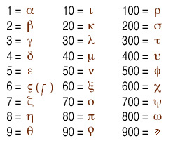
The Greek system of numerals, as used in New Testament and early Byzantine times, was at least more compact than the Roman, though it (like all ancient systems) lacked the zero and so was not really suitable for advanced computation. The 24 letters of the alphabet were all used as numerals, as were three obsolete letters, bringing the total to 27. This allowed the representation of all numbers less than 1000 using a maximum of three symbols, as shown at right:
Thus 155, for instance, would be written as rne; 23 would be kg, etc.
Numbers over 1000 could also be expressed, simply by application of a divider. So the number 875875 would become woe,woe'. Note that this allowed the Greeks to express numbers actually larger than the largest "named" number in the language, the myriad (ten thousand). (Some deny this; they say the system only allowed four digits, up to 9999. This may have been initially true, but both Archimedes and Apollonius were eventually forced to extend the system -- in different and conflicting ways. In practice, it probably didn't come up very often.)
Of course, this was a relatively recent invention. The Mycenaean Greeks
in the Linear B tablets had used a completely different system:
| for digits, - for tens, o for hundreds,
![]() for thousands.
So, for instance, the number we would now express as 2185 would
have been expressed in Pylos as
for thousands.
So, for instance, the number we would now express as 2185 would
have been expressed in Pylos as
![]()
![]() o====|||||. But
this system, like all things about Linear B, seems to have been
completely forgotten by classical times.
o====|||||. But
this system, like all things about Linear B, seems to have been
completely forgotten by classical times.
A second system, known as the "Herodian," or "Attic," was
still remembered in New Testament times, though rarely if ever used. It
was similar to Roman numerals in that it used symbols for particular numbers
repeatedly -- in this system, we had
I = 1
D = 10
H = 100
X = 1000
M = 10000
(the letters being derived from the first words of the names of the numbers).
However, like Roman numerals, the Greeks added a trick to simplify, or at least compress, the symbols. To the above five symbols, they added P for five -- but it could be five of anything -- five ones, five tens, five hundreds, with a subscripted figure showing which it was. In addition, in practice, the number was often written as G rather than P to allow numbers to be fitted under it. So, e.g., 28,641 would be written as
M M GX X X X GH H D D D D I
In that context, it's perhaps worth noting that the Greek verb for "to count" is pempw, related to pente, five. The use of a system such as this was almost built into the language. But its sheer inconvenience obviously helped assure the later success of the Ionian system, which -- to the best of my knowledge -- is the one followed in all New Testament manuscripts which employ numerals at all.
And it should be remembered that these numerals were very widely used. Pick up a New Testament today and look up the "Number of the Beast" in Rev. 13:18 and you will probably find the number spelled out (so, e.g., in Merk, NA27, and even Westcott and Hort; Bover and Hodges and Farstad uses the numerals). It's not so in the manuscripts; most of them use the numerals (and numerals are even more likely to appear in the margins, e.g. for the Eusebian tables). This should be kept in mind when assessing variant readings. Since, e.g., s and o can be confused in most scripts, one should be alert to scribes confusing these numerals even when they would be unlikely to confuse the names of the numbers they represent. O. A. W. Dilke in Greek and Roman Maps (a book devoted as much to measurement as to actual maps) notes, for instance, that "the numbers preserved in their manuscripts tend to be very corrupt" (p. 43). Numbers aren't words; they are easily corrupted -- and, because they have little redundancy, if a scribe makes a copying error, a later scribe probably can't correct it. It's just possible that this might account for the variant 70/72 in Luke 10:1, for instance, though it would take an unusual hand to produce a confusion in that case.
There is at least one variant, in fact, where a confusion involving numerals is nearly a certainty -- Acts 27:37. Simply reading the UBS text here, which spells out the numbers, is flatly deceptive. One should look at the numerals. The common text here is
![]()
In B, however, supported by the Sahidic Coptic (which of course uses its own number system), we have
![]()
Which would become
![]()
This latter reading is widely rejected. I personally think it deserves respect. The difference, of course, is only a single omega, added or deleted. But I think dropping it, which produces a smoother reading, is more likely. Also, while much ink has been spilled justifying the possibility of a ship with 276 people aboard (citing Josephus, e.g., to the effect that the ship that took him to Rome had 600 people in it -- a statement hard to credit given the size of all known Roman-era wrecks), possible is not likely.
We should note some other implications of this system -- particularly for gematria (the finding of mathematical equivalents to a text). Observe that there are three numerals -- those for 6, 90, and 900 -- which will never be used in a text (unless one counts a terminal sigma, and that doesn't really count). Other letters, while they do occur, are quite rare (see the section on Cryptography for details), meaning that the numbers corresponding to them are also rare. The distribution of available numbers means that any numeric sum is possible, at least if one allows impossible spellings, but some will be much less likely than others. This might be something someone should study, though there is no evidence that it actually affects anything.
Of course, Greek mathematics was not confined simply to arithmetic. Indeed, Greek mathematics must be credited with first injecting the concept of rigour into mathematics -- for all intents and purposes, turning arithmetic into math. This is most obvious in geometry, where they formalized the concept of the proof.
According to Greek legend, which can no longer be verified, it was the famous Thales of Miletus who gave some of the first proofs, showing such things as the fact that a circle is bisected by a diameter (i. e. there is a line -- in fact, an infinite number of lines -- passing through the center of the circle which divides the area of a circle into equal halves), that the base angles of an isoceles triangle (the ones next to the side which is not the same length as the other two) are equal, that the vertical angles between two intersecting lines (that is, either of the two angles not next to each other) are equal, and that two triangles are congruent if they have two equal angles and one equal side. We have no direct evidence of the proof by Thales -- everything we have of his work is at about third hand -- but he was certainly held up as an example by later mathematicians.
The progress in the field was summed up by Euclid (fourth/third century), whose Elements of geometry remains fairly definitive for plane geometry even today.
Euclid also produces the (surprisingly easy) proof that the number of primes is infinite -- giving, incidentally, a nice example of a proof by contradiction, a method developed by the Greeks: Suppose there is a largest prime (call it p). So take all the primes: 2, 3, 5, 7, ... p. Multiply all of these together and add one. This number, since it is one more than a multiple of all the primes, cannot be divisible by any of them. It is therefore either prime itself or a multiple of a prime larger than p. So p cannot be the largest prime, which is a contradiction.
A similar proof shows that the square root of 2 is irrational -- that is, it cannot be expressed as the ratio of any two whole numbers. The trick is to express the square root of two as a ratio and reduce the ratio p/q to simplest form, so that p and q have no common factors. So, since p/q is the square root of two, then (p/q)2 = 2. So p2=2q2. Since 2q2 is even, it follows that p2 is even. Which in turn means that p is even. So p2 must be divisible by 4. So 2q2 must be divisible by 4, so q2 must be divisible by 2. And, since we know the square root of 2 is not a whole number, that means that q must be divisible by 2. Which means that p and q have a common factor of 2. This contradiction proves that there is no p/q which represents the square root of two.
This is one of those crucial discoveries. The Egyptians, as we shall see, barely understood fractions. The Babylonians did understand them, but had no theory of fractions. They could not step from the rational numbers (fractions) to the irrational numbers (endless non-repeating decimals). The Greeks, with results such as the above, not only invented mathematical logic -- crucial to much that followed, including statistical analysis such as many textual critics used -- but also, in effect, the whole system of real numbers.
The fact that the square root of two was irrational had been known as early as the time of Pythagoras, but the Pythagoreans hated the fact and tried to hide it. Euclid put it squarely in the open. (Pythagoras, who lived in the sixth century, of course, did a better service to math in introducing the Pythagorean Theorem. This was not solely his discovery -- several other peoples had right triangle rules -- but Pythagoras deserves credit for proving it analytically.)
Relatively little of Euclid's work was actually original; he derived most of it from earlier mathematicians, and often the exact source is uncertain (Boyer, in going over the history of this period, seems to spend about a quarter of his space discussing how particular discoveries are attributed to one person but perhaps ought to be credited to someone else; I've made no attempt to reproduce all these cautions and credits). That does not negate the importance of his work. Euclid gathered it, and organized it, and so allowed all that work to be maintained. But, in another sense, he did more. The earlier work had been haphazard. Euclid turned it into a system. This is crucial -- equivalent, say, to the change which took place in biology when species were classified into genuses and families and such. Before Euclid, mathematics, like biology before Linnaeus, was essentially descriptive. But Euclid made it a unity. To do so, he set forth ten postulates, and took everything from there.
Let's emphasize that. Euclid set forth ten postulates (properly, five axioms and five postulates, but this is a difference that makes no difference). Euclid, and those on whom he relied, set forth what they knew, and defined their rules. This is the fundamental basis to all later mathematics -- and is something textual critics still haven't figured out! (Quick -- define the Alexandrian text!)
Euclid in fact hadn't figured everything out; he made some assumptions he didn't realize he was making. Also, since his time, it has proved possible to dispense with certain of his postulates, so geometry has been generalized. But, in the realm where his postulates (stated and unstated) apply, Euclid remains entirely correct. The Elements is still occasionally used in math classes today. And the whole idea of postulates and working from them is essential in mathematics. I can't say it often enough: this was the single most important discovery in the history of math, because it defines rigour. Euclid's system, even though the individual results preceded him, made most future maths possible.
The sufficiency of Euclid's work is shown by the extent to which it eliminated all that came before. There is only one Greek mathematical work which survives from the period before Euclid, and it is at once small and very specialized -- and survived because it was included in a sort of anthology of later works. It's not a surprise, of course, that individual works have perished (much of the work of Archimedes, e.g., has vanished, and much of what has survived is known only from a single tenth-century palimpsest, which obviously is both hard to interpret and far removed from the original). But all of it? Clearly Euclid was considered sufficient.
And for a very long time. The first printed edition of Euclid came out in 1482, and it is estimated that over a thousand editions have been published since; it has been claimed that it is the most-published book of all time other than the Bible.
Not that the Greeks stopped working once Euclid published his work.
Apollonius, who did most of the key work on conic sections, came later,
as did Eratosthenes, perhaps best remembered now for accurately measuring
the circumference of the earth but also noteworthy for inventing the
"sieve" that bears his name for finding prime numbers.
And, their greatest mathematician was no more than a baby when Euclid
wrote the Elements. Archimedes -- surely the greatest scientific
and mathematical genius prior to Newton, and possibly even Newton's
equal had he had the data and tools available to the latter -- was
scientist, engineer, the inventor of mathematical physics, and
a genius mathematician. In the latter area, several
of his accomplishments stand out. One is his work on large numbers in
The Sand Reckoner, in which he set out to determine the maximum
number of sand grains the universe might possibly hold. To do this, he
had to invent what amounted to exponential notation. He also, in so
doing, produced the notion of an infinitely extensible number system.
The notion of infinity was known to the Greeks, but had been the subject
of rather unfruitful debate. Archimedes gave them many of the tools they
needed to address some of the problems -- though few later scholars made
use of the advances.
Archimedes also managed, in one step, to create one of the tools that would turn into the calculus (though he didn't know it) and to calculate an extremely accurate value for p, the ratio of the circumference of a circle to its diameter. The Greeks were unable to find an exact way to calculate the value -- they did not know that p is irrational; this was not known with certainty until Lambert proved it in 1761. The only way the Greeks could prove a number irrational was by finding the equivalent of an algebraic equation to which it was a solution. They couldn't find such, for the good and simple reason that there is no such equation. This point -- that p is what we now call a transcendental number -- was finally proved by Ferdinand Lindemann in 1882.
Archimedes didn't know that p is irrational, but he did know he didn't know how to calculate it. He had no choice but to seek an approximation. He did this by the beautifully straightforward method of inscribed and circumscribed polygons. The diagram at right shows how this works: The circumference of the circle is clearly greater than the circumference of the square inscribed inside it, and less than the square circumscribed around it. If we assume the circle has a radius of 1 (i.e. a diameter of 2), then the perimeter of the inner square can be shown to be 4 times the square root of two, or about 5.66. The perimeter of the outer square (whose sides are the same length as the diameter of the circle) is 8. Thus the circumference of the circle, which is equal to 2p, is somewhere between 5.66 and 8. (And, in fact, 2p is about 6.283, so Archimedes is right). But now notice the second figure, in which an octagon has been inscribed and circumscribed around the circle. It is obvious that the inner octagon is closer to the circle than the inner square, so its perimeter will be closer to the circumference of the circle while still remaining less. And the outer octagon is closer to the circle while still remaining greater.
If we repeat this procedure, inscribing and circumscribing polygons with more and more faces, we come closer and closer to "trapping" the value of p. Archimedes, despite having only the weak Greek mathematical notation at his disposal, managed to trap the value of p as somewhere between 223/71 (3.14085) and 220/70 (3.14386). The first of these values is about .024% low of the actual value of p; the latter is about .04% high; the median of the two is accurate to within .008%. That is an error too small to be detected by any measurement device known in Archimedes's time; there aren't many outside an advanced science lab that could detect it today.
Which is nice enough. But there is also a principle there. Archimedes couldn't demonstrate it, because he hadn't the numbering system to do it -- but his principle was to add more and more sides to the inscribing and circumscribing polygons. Suppose he had taken infinitely many sides? In that case, the inscribing and circumscribing polygons would have merged with the circle, and he would have had the exact value of p. This is the principle of the limit, and it is the basis on which the calculus is defined. It is sometimes said that Archimedes would have invented the calculus had he had Arabic numerals. This statement is too strong. But he might well have created a tool which could have led to the calculus.
An interesting aspect of Greek mathematics was their search for solutions even to problems with no possible use. A famous example is the attempt to "square the circle" -- starting from a circle, to construct a square with the same area using nothing but straight edge and compass. This problem goes back all the way to Anaxagoras, who died in 428 B.C.E. The Greeks never found an answer to that one -- it is in fact impossible using the tools they allowed themselves -- but the key point is that they were trying for general and theoretical rather than practical and specific solutions. That's the key to a true mathematics.
In summary, Greek mathematics was astoundingly flexible, capable of handling nearly any engineering problem found in the ancient world. The lack of Arabic numbers made it difficult to use that knowledge (odd as it sounds, it was easier back then to do a proof than to simply add up two numbers in the one million range). But the basis was there.
To be sure, there was a dark -- or at least a goofy -- side to Greek mathematics. Plato actually thought mathematics more meaningful than data -- in the Republic, 7.530B-C -- he more or less said that, where astronomical observations and mathematics disagreed, too bad for the facts. Play that game long enough, and you'll start distorting the math as well as the facts....
The goofiness is perhaps best illustrated by some of the uses to which mathematics was put. The Pythagoreans were famous for their silliness (e.g. their refusal to eat beans), but many of their nutty ideas were quasi-mathematical. An example of this is their belief that 10 was a very good and fortunate number because it was equal to 1+2+3+4. Different Greek schools had different numerological beliefs, and even good mathematicians could fall into the trap; Ptolemy, whose Almagest was a summary of much of the best of Greek math, also produced the Tetrabiblos of mystical claptrap. The good news is, relatively few of the nonsense works have survived, and as best I can tell, none of the various superstitions influenced the NT writers. The Babylonians also did this sort of thing -- they in fact kept it all secret, concealing some of their knowledge with cryptography, and we at least hear of this sort of mystic knowledge in the New Testament, with Matthew's mention of (Babylonian) Magi -- but all he seems to have cared was that they had secret knowledge, not what that knowledge was.
At least the Greek had the sense to separate rigourous from silly, which many other people did not. Maybe they were just frustrated with the difficulty of achieving results. The above description repeatedly laments the lack of Arabic numbers -- i.e. with positional notation and a zero. This isn't just a matter of notational difficulty; without a zero, you can't have the integers, nor negative numbers, let alone the real and complex numbers that let you solve all algebraic equations. Arabic numbers are the mathematical equivalent of an alphabet, only even more essential. The advantage they offer is shown by an example we gave above: The determination of p by means of inscribed and circumscribed polygons. Archimedes could manage only about three decimal places even though he was a genius. François Viète (1540-1603) and Ludolph van Ceulen (1540-1610) were not geniuses, but they managed to calculate p to ten and 35 decimal places, respectively, using the method of Archimedes -- and they could do it because they had Arabic numbers.
The other major defect of Greek mathematics was that the geometry was not analytic. They could draw squares, for instance -- but they couldn't graph them; they didn't have cartesian coordinates or anything like that. Indeed, without a zero, they couldn't draw graphs; there was no way to have a number line or a meeting point of two axes. This may sound trivial -- but modern geometry is almost all analytic; it's much easier to derive results using non-geometric tools. It has been argued that the real reason Greek mathematics stalled in the Roman era was not lack of brains but lack of scope: There wasn't much else you could do just with pure geometric tools.
The lack of a zero (and hence of a number line) wasn't just a problem for the Greeks. We must always remember a key fact about early mathematics: there was no universal notation; every people had to re-invent the whole discipline. Hence, e.g., though Archimedes calculated the value of p to better than three decimal places, we find 1 Kings 7:23, in its description of the bronze sea, rounding off the dimensions to the ratio 30:10. (Of course, the sea was built and the account written before Archimedes. More to the point, both measurements could be accurate to the single significant digit they represent without it implying a wrong value for p -- if, e.g., the diametre were 9.7 cubits, the circumference would be just under 30.5 cubits. It's also worth noting that the Hebrews at this time were probably influenced by Egyptian mathematics -- and the Egyptians did not have any notion of number theory, and so, except in problems involving whole numbers or simple fractions, could not distinguish between exact and approximate answers.)
Still, Hebrew mathematics was quite primitive. There really wasn't much there apart from the use of the letters to represent numbers. I sometimes wonder if the numerical detail found in the so-called "P" source of the Pentateuch doesn't somehow derive from the compilers' pride in the fact that they could actually count that high!
Much of what the Hebrews did know may well have been derived from the Babylonians, who had probably the best mathematics other than the Greek; indeed, in areas other than geometry, the Babylonians were probably stronger. And they started earlier; we find advanced mathematical texts as early as 1600 B.C.E., with some of the basics going all the way back to the Sumerians, who seem to have been largely responsible for the complex 10-and-60 notation used in Babylon. How much of this survived to the time of the Chaldeans and the Babylonian Captivity is an open question; Ifrah says the Babylonians converted their mathematics to a simpler form around 1500 B.C.E., but Neugebauer, generally the more authoritative source, states that their old forms were still in use as late as Seleucid times. Trying to combine the data leads me to guess the Chaldeans had a simpler form, but that the older, better maths were retained in some out-of-the-way places.
It is often stated that the Babylonians used Base 60. This statement is somewhat deceptive. The Babylonians used a mixed base, partly 10 and partly 60. The chart below, showing the cuneiform symbols they used for various numbers, may make this clearer.

This mixed system is important, because base 60 is too large to be a comfortable base -- a multiplication table, for instance, has 3600 entries, compared to 100 entries in Base 10. The mixed notation allowed for relatively simple addition and multiplication tables -- but also for simple representation of fractions.
For very large numbers, they had still another system -- a partial positional notation, based on using a space to separate digits. So, for instance, if they wrote | || ||| (note the spaces between the wedges), that would mean one times 60 squared (i.e. 3600) plus two times 60 plus three, or 3723. This style is equivalent to our 123 = one times ten squared plus two times ten plus three. The problem with this notation (here we go again) is that it had no zero; if they wrote IIII II, say, there was no way to tell if this meant 14402 (4x602+0x60+2) or 242 (4x60+2). And there was no way, in this notation, to represent 14520 (4x602+2x60+0). (The Babylonians did eventually -- perhaps in or shortly before Seleucid times -- invent a placeholder to separate the two parts, though it wasn't a true zero; they didn't have a number to represent what you got when you subtracted, e.g., nine minus nine.)
On the other hand, it did allow representation of fractions, at least as long as they had no zero elements: Instead of using positive powers of 60 (602=3600, 601=60, etc.), they could use negative powers -- 60-1=1/60, 60-2=1/3600, etc. So they could represent, say, 1/15 (=4/60) as ||||, or 1/40 (=1/60 + 30/3600) as I <<<, making them the only ancient people with a true fractional notation.
Thus it will be seen that the Babylonians actually used Base 10 -- but generally did calculations in Base 60.
There is a good reason for the use of Base 60, the reason being that 60 has so many factors: It's divisible by 2, 3, 4, 5, 6, 12, 15, 20, and 30. This means that all fractions involving these denominators are easily expressed (important, in a system where decimals were impossible due to the lack of a zero and even fractions didn't have a proper means of notation). This let the Babylonians set up fairly easy-to-use computation tables. This proved to be so much more useful for calculating angles and fractions that even the Greeks took to expressing ratios and angles in Base 60, and we retain a residue of it today (think degrees/minutes/seconds). The Babylonians, by using Base 60, were able to express almost every important fraction simply, making division simple; multiplication by fractions was also simplified. This fact also helped them discover the concept (though they wouldn't have understood the term) of repeating decimals; they had tables calculating these, too.
Base 60 also has an advantage related to human physiology. We can count up to five at a glance; to assess numbers six or greater required counting. So, given the nature of the cuneiform numbers expressing 60 or 70 by the same method as 50 (six or seven pairs of brackets as opposed to five) would have required more careful reading of the results. As it was, numbers could be read quickly and accurately. A minor point, but still an advantage.
Nor were the Babylonians limited to calculating fractions. The Babylonians calculated the square root of two to be roughly 1.414213, an error of about one part in one million! (As a rough approximation, they used 85/60, or 1.417, still remarkably good.) All of this was part of their approach to what we would call algebra, seeking the solution to various types of equations. Many of the surviving mathematics tablets are what my elementary school called "story problems" -- a problem described, and then solved in such a way as to permit general solutions to problems of the type.
There were theoretical complications, to be sure. Apart from the problem that they sometimes didn't distinguish between exact and approximate solutions, their use of units would drive a modern scientist at least half mad -- there is, for instance, a case of a Babylonian tablet adding a "length" to an "area." It has been proposed that "length" and "width" came to be the Babylonian term for variables, as we would use x, y, and z. This is possible -- but the result still permits confusion and imprecision.
We should incidentally look at the mathematics of ancient Mari, since it is believed that many of the customs followed by Abraham came from that city. Mari appears to have used a modification of the Babylonian system that was purely 10-based: It used a system exactly identical to the Babylonian for numbers 1-59 -- i.e. vertical wedges for the numbers 1-9, and chevrons ( < ) for the tens. So <<II, e.g., would represent 22, just as in Babylonian.
The first divergence came at 60. The Babylonians adopted a different symbol here, but in Mari they just went on with what they were doing, using six chevrons for 60, seven for seventy, etc. (This frankly must have been highly painful for scribes -- not just because it took 18 strokes, e.g. to express the number 90, but because 80 and 90 are almost indistinguishable).
For numbers in the hundreds, they would go back to the symbol used for ones, using positions to show which was which -- e.g. 212 would be ||<||. (Interestingly, they used the true Babylonian notation for international and "scientific" documents.) But they did not use this to develop a true positional notation (and they had no zero); rather, they had a complicated symbol for 1000 (four parallel horizontal wedges, a vertical to their right, and another horizontal to the right of that), which they used as a separator -- much as we would use the , in the number 1,000 -- and express the number of thousands with the same old unit for ones.
This system did not, however, leave any descendants that we know of; after Mari was destroyed, the other peoples in the area went back to the standard Babylonian/Akkadian notation.
The results of Babylonian math are quite sophisticated; it is most unfortunate that the theoretical work could not have been combined with the Greek concept of rigour. The combination might have advanced mathematics by hundreds of years. It is a curious irony that Babylonian mathematics was immensely sophisticated but completely pointless; like the Egyptians and the Hebrews, they had no theory of numbers, and so while they could solve problems of particular types with ease, they could not generalize to larger classes of problems. Which may not sound like a major drawback, but realize what this means: If the parameters of a problem changed, even slightly, the Babylonians had no way to know if their old techniques would accurately solve it or not.
None of this matters now, since we have decimals and Arabic numerals. Little matters even to Biblical scholars, even though, as noted, Hebrew math probably derives from Babylonian (since the majority of Babylonian tablets come from the era when the Hebrew ancestors were still under Mesopotamian influence, and they could have been re-exposed during the Babylonian Captivity, since Babylonian math survived until the Seleudid era) or perhaps Egyptian; there is little math in the Old Testament, and what there is has been "translated" into Hebrew forms. Nonetheless the pseudo-base of 60 has genuine historical importance: The 60:1 ratio of talent: mina: shekel is almost certainly based on the Babylonian use of Base 60.
Much of Egyptian mathematics resembles the Babylonian in that it seeks directly for the solution, rather than creating rigourous methods, though the level of sophistication is much less.
A typical example of Egyptian dogmatism in mathematics is their insistence that fractions could only have unitary numerators -- that is, that 1/2, 1/3, 1/4, 1/5 were genuine fractions, but that a fraction such a 3/5 was impossible. If the solution to a problem, therefore, happened to be 3/5, they would have to find some alternate formulation -- 1/2 + 1/10, perhaps, or 1/5 + 1/5 + 1/5, or even 1/3 + 1/4 + 1/60. Thus a fraction had no unique expression in Egyptian mathematics -- making rigour impossible; in some cases, it wasn't even possible to tell if two people had come up with the same answer to a problem!
Similarly, they had a fairly accurate way of calculating the area of a circle (in modern terms, 256/81, or about 3.16) -- but they didn't define this in terms of a number p (their actual formula was (8d/9)2, where d is the diameter), and apparently did not realize that this number had any other uses such as calculating the circumference of the circle.
Egyptian notation was of the basic count-the-symbols type we've seen, e.g., in Roman and Mycenean numbers. In heiroglyphic, the units were shown with the so-very-usual straight line |. Tens we a symbol like an upside-down U -- ∩. So 43, for instance, would be ∩∩∩∩III. For hundreds, they used a spiral; a (lotus?) flower and stem stood for thousands. An image of a bent finger stood for ten thousands. A tadpole-like creature represented hundred thousands. A kneeling man with arms upraised counted millions -- and those high numbers were used, usually in boasts of booty captured. They also had four symbols for fractions: special symbols for 1/2, 2/3, and 3/4, plus the generic reciprocal symbol, a horizontal oval we would read a "one over" So some typical fractions would be
| 1/4: ⊂⊃ II II | 1/6: ⊂⊃ III III | 1/16: ⊂⊃ ∩II IIII |
It will be seen that there is no way to express, say, 2/5 in this system; it would be either 1/5+1/5 or, since the Egyptians don't seem to have liked repeating fractions either, something like 1/3+1/15. (Except that they seem to have preferred to put the smaller fraction first, so this would be written 1/15+1/3.)
The Egyptians actually had a separate fractional notation for volume measure, fractions-of-a-heqat. I don't think this comes up anywhere we would care about, so I'm going to skip trying to explain it. Nonetheless, it was a common problem in ancient math -- the inability to realize that numbers were numbers. It often was not realized that, say, three drachma were the same as three sheep were the same as three logs of oil. Various ancient systems had different number-names, or at least three different symbols, for all these numbers -- as if we wrote "3 sheep" but "III drachma." We have vestiges of this today -- consider currency, where instead of saying, e.g., "3 $," we write "$3" -- a significant notational difference.
We also still have some hints of the ancient problems with fractions, especially in English units (those on the metric system have largely solved this): Instead of measuring a one and a half pound loaf of bread as weighing "1.5 pounds," it will be listed as consisting of "1 pound 8 ounces." A quarter of a gallon of milk is not ".25 gallon"; it's "1 quart." (This is why scientists use the metric system!) This was even more common in ancient times, when fractions were so difficult: Instead of measuring everything in shekels, say, we have shekel/mina/talent, and homer/ephah, and so forth.
Even people who use civilized units of measurement often preserve the ancient fractional messes in their currency. The British have rationalized pounds and pence and guineas -- but they still have pounds and shillings and pence. Americans use dollars and cents, with the truly peculiar notation that dollars are expressed (as noted above) "$1.00," while cents are "100 ¢"; the whole should ideally be rationalized. Germans have marks and pfennig. And so forth. Similarly, we have a completely non-decimal time system; 1800 seconds are 30 minutes or 1/2 hour or 1/48 day. Oof!
We of course are used to these funny cases. But it should alsways be kept in mind that the ancients used this sort of system for everything -- and had even less skill than we in converting.
But let's get back to Egyptian math....
The hieratic/demotic had a more compact, though more complicated, system than hieroglyphic. I'm not going to try to explain this, just show the various symbols as listed in figure 14.23 (p. 176) of Ifrah. This is roughly the notation used in the Rhind Papyrus, though screen resolution makes it hard to display the strokes clearly.
This, incidentally, does much to indicate the difficulty of ancient
notations. The Egyptians, in fact, do not seem even to have had a concept
of general "multiplication"; their method -- which is ironically
similar to a modern computer -- was the double-and-add. For example, to
multiply 23 by 11 (which we could either do by direct multiplication or
by noting that 11=10+1, so
23x11 = 23x(10+1)=23x10 + 23x1 =230+23=253), they
would go through the following steps:
23x1 = 23
23x2 = 46
23x4 = 92
23x8 = 184
and 11=8+2+1
so 23x11 = (23x8) + (23x2) + (23+1) = 184 + 46 + 23 = 253
This works, but oy. A problem I could do by inspection takes six major steps, with all the chances for error that implies.
The same, incidentally, is true in particular of Roman numerals.
This is thought to be the major reason various peoples invented the
abacus: Even addition was very difficult in their systems, so they
didn't do actual addition; they counted out the numbers on the abacus
and then translated them back into their notation.
That description certain seems to fit the Hebrews. Hebrew mathematics frankly makes one wonder why God didn't do something to educate these people. Their mathematics seems to have been even more primitive than the Romans'; there is nothing original, nothing creative, nothing even particularly efficient. It's almost frightening to think of a Hebrew designing Solomon's Temple, for instance, armed with all the (lack of) background on stresses and supports that a people who still lived mostly in tents had at their disposal. (One has to suspect that the actual temple construction was managed by either a Phoenician or an Egyptian.)
The one thing that the Hebrews could call their own was their numbering system (and even that probably came from the Phoenicians along with the alphabet). They managed to produce a system with most of the handicaps, and few of the advantages, of both the alphabetic systems such as the Greek and the cumulative systems such as the Roman. As with the Greeks, they used letters of the alphabet for numbers -- which meant that numbers could be confused with words, so they often prefixed ' or a dot over the number to indicate that it was a numeral. But, of course, the Hebrew alphabet had only 22 letters -- and, unlike the Greeks, they did not invoke other letters to supply the lack (except that a few texts use the terminal forms of the letters with two shapes, but this is reportedly rare). So, for numbers in the high hundreds, they ended up duplicating letters -- e.g. since one tau meant 400, two tau meant 800. Thus, although the basic principle was alphabetic, you still had to count letters to an extent.
The basic set of Hebrew numbers is shown at right.
An interesting and uncertain question is whether this notation preceded,
supplanted, or existed alongside Aramaic numerals.
The Aramaeans seem to have used a basic additive system. The numbers
from one to nine were simple tally marks, usually grouped in threes --
e.g. 5 would be || ||| (read from right to left, of course);
9 would be ||| ||| |||. For 10 they used a curious pothook,
perhaps the remains of a horizontal bar, something like a ∼ or ∩
or ![]() . They also had
a symbol for 20, apparently based on two of these things stuck together;
the result often looked rather like an Old English yogh
(
. They also had
a symbol for 20, apparently based on two of these things stuck together;
the result often looked rather like an Old English yogh
(![]() ) or perhaps
≈. Thus the number 54 would be written
| ||| ∼
) or perhaps
≈. Thus the number 54 would be written
| ||| ∼![]()
![]() .
.
There is archaeological evidence for both forms. Coins of Alexander Jannaeus (first century B.C.E.) use alphabetic numbers. But we find Aramaic numbers among the Dead Sea Scrolls. This raises at least a possibility that the number form one used depended upon one's politics. The Jews at Elephantine (early Persian period) appear to have used Aramaic numbers -- but they of course were exiles, and living in a period before Jews as a whole had adopted Aramaic. On the whole, the evidence probably favors the theory that Aramaic numbering preceded Hebrew, but we cannot be dogmatic. In any case, Hebrew numbers were in use by New Testament times; we note, in fact, that coins of the first Jewish Revolt -- which are of course very nearly contemporary with the New Testament books -- use the Hebrew numerals.
There is perhaps one other point we should make about mathematics,
and that is the timing of the introduction of Arabic numerals. An early
manuscript of course cannot contain such numbers; if it has numerals
(in the Eusebian apparatus, say), they will be Greek (or Roman, or
something). A late minuscule, however, can contain Arabic numbers --
and, indeed, many have pages numbered in this way.
Arabic numerals underwent much change over the years. The graphic at right barely sketches the evolution. The first three samples are based on actual manuscripts (in the first case, based on scans of the actual manuscript; the others are composite).
The first line is from the Codex Vigilanus, generally regarded as the earliest use of Arabic numerals in the west (though it uses only the digits 1-9, not the zero). It was written, not surprisingly, in Spain, which was under Islamic influence. The codex (Escurial, Ms. lat. d.1.2) was copied in 976 C. E. by a monk named Vigila at the Abelda monastery. The next several samples are (based on the table of letterforms in Ifrah) typical of the next few centuries. Following this, I show the evolution of forms described in E. Maunde Thompson, An Introduction to Greek and Latin Paleography, p. 92. Thompson notes that Hindu/Arabic numerals were used mostly in mathematical works until the thirteenth century, becoming universal in the fourteenth century. Singer, p. 175, describes a more complicated path: Initially they were used primarily in connection with the calendar. The adoption of Arabic numerals for mathematics apparently can be credited to one Leonardo of Pisa, who had done business in North Africa and seen the value of the system. He'll perhaps sound more familiar if we note that he was usually called "Fibonacci," the "Son of Bonaccio" -- now famous for his series (0, 1, 1, 2, 3, 5, 8...) in which each term is the sum of the previous two. But his greatest service to mathematics was his support of modern notation. In 1202 he put forth the Book of the Abacus, a manual of calculation (which also promoted the horizontal stroke - to separate the numerators and denominators of fractions, though his usage was, by modern standards, clumsy, and it took centuries for this notation to catch on). The use of Arabic numerals was further encouraged when the Yorkshireman John Holywood (died 1250) produced his own book on the subject, which was quote popular; Singer, p. 173, reports that Holywood "did more to introduce the Arabic notation than any other." Within a couple of centuries, they were commonly used. In Chaucer's Treatise on the Astrolabe I.7, for instance, addressed to his ten-year-old son, he simply refers to them as "noumbers of augrym" -- i.e., in effect, abacus numbers -- and then proceeds to scatter them all through the text.) If someone has determined the earliest instance of Arabic numbers in a Biblical manuscript, I confess I do not know what it is.
Most other modern mathematical symbols are even more recent. The symbols + and - for addition and subtraction, for instance, are first found in print in Johann Widman's 1489 publication Rechnung uff allen Kauffmanschafften. (Prior to that, it was typical to use the letters p and m.) The = sign seems to go back to England's Robert Recorde (died 1558), who published several works dating back to 1541 -- though Recorde's equality symbol was much wider than ours, looking more like ====. The notation became general about a century later. The modern notation of variables (and parameters) can be credited to François Viète (1540-1603), who also pushed for use of decimal notation in fractions and experimented with notations for the radix point (what we tend to call the "decimal point," but it's only a decimal point in Base 10; in Base 2, e.g., it's the binary point. In any case, it's the symbol for the division between whole number and fractional parts -- usually, in modern notation, either a point or a comma).
The table below briefly shows the forms of numerals in some of the languages in which New Testament versions exist. Some of these probably require comment -- e.g. Coptic numerals are theoretically based on the Greek, but they had a certain amount of time to diverge. Observe in particular the use of the chi-rho for 900; I assume this is primarily a Christian usage, but have not seen this documented. Many of the number systems (e.g. the Armenian) have symbols for numbers larger than 900, but I had enough trouble trying to draw these clearly!
Addendum: Textual Criticism of Mathematical Works
Most ancient mathematical documents exist in only a single copy (e.g. the Rhind Papyrus is unique), so any textual criticism must proceed by conjecture. And this is in fact trickier than it sounds. If an ancient document adds, say, 536 and 221 and reaches a total of 758 instead of the correct 757, can we automatically assume the document was copied incorrectly? Not really; while this is a trivial sum using Arabic numerals, there are no trivial sums in most ancient systems; they were just too hard to use!
But the real problems are much deeper. Copying a mathematical manuscript is a tricky proposition indeed. Mathematics has far less redundancy than words do. In words, we have "mis-spellings," e.g., which formally are errors but which usually are transparent. In mathematics -- it's right or it's wrong. And any copying error makes it wrong. And, frequently, you not only have to copy the text accurately, but any drawings. And labels to the drawings. And the text that describes those labels. To do this right requires several things not in the standard scribe's toolkit -- Greek mathematics was built around compass and straight edge, so you had to have a good one of each and the ability to use it. Plus the vocabulary was inevitably specialized.
The manuscripts of Euclid, incidentally, offer a fascinating parallel with the New Testament tradition, especially as the latter was seen by Westcott and Hort. The majority of manuscripts belong to a single type, which we know to be recensional: It was created by the editor Theon. Long after Euclid was rediscovered, a single manuscript was found in the Vatican, containing a text from a different recension. It is generally thought to be earlier. Such papyrus scraps as are available generally support the Vatican manuscript, without by any means agreeing with it completely. Still, it seems clear that the majority text found in Theon has been somewhat smoothed and prettied up, though few of the changes are radical and it sometimes seems to retain the correct text where the Vatican type has gone astray.
Bibliography to the section on Ancient Mathematics
The study of ancient mathematics is difficult; one has to understand language and mathematics, and have the ability to figure out completely alien ways of thinking. I've consulted quite a few books to compile the above (e.g. Chadwick's publications on Linear B for Mycenaean numerals), and read several others in a vain hope of learning something useful, but most of the debt is to five books (which took quite a bit of comparing!). The "select bibliography:"
In addition, if you're interested in textual criticism of mathematical works, you might want to check Thomas L. Heath's translation of Euclid (published by Dover), which includes an extensive discussion of Euclid's text and Theon's recension, as well as a pretty authoritative translation with extensive notes.
"Assuming the solution" is a mathematical term for a particularly vicious fallacy (which can easily occur in textual criticism) in which one assumes something to be true, operates on that basis, and then "proves" that (whatever one assumed) is actually the case. It's much like saying something like "because it is raining, it is raining." It's just fine as long as it is, in fact, actually raining -- but if it isn't, the statement is inaccurate. In any case, it doesn't have any logical value. It is, therefore, one of the most serious charges which can be levelled at a demonstration, because it says that the demonstration is not merely incomplete but is founded on error.
As examples of assuming the solution, we may offer either Von Soden's definition of the I text or Streeter's definition of the "Cæsarean" text. Both, particularly von Soden's, are based on the principle of "any non-Byzantine reading" -- that is, von Soden assumes that any reading which is not Byzantine must be part of the I text, and therefore the witness containing it must also be part of the I text.
The problem with this is that it means that everything can potentially be classified as an I manuscript, including (theoretically) manuscripts which have not a single reading in common at points of variation. It obviously can include manuscripts which agree only in Byzantine readings. This follows from the fact that most readings are binary (that is, only two readings are found in the tradition). One reading will necessarily be Byzantine. Therefore the other is not Byzantine. Therefore, to von Soden, it was an I reading. It doesn't matter where it actually came from, or what sort of reading it is; it's listed as characteristic of I.
This sort of error has been historically very common in textual criticism. Critics must strive vigorously to avoid it -- to be certain they do not take something on faith. Many results of past criticism were founded on assuming the solution (including, e.g., identifying the text of P46 and B with the Alexandrian text in Paul). All such results need to be re-verified using definitions which are not self-referencing.
Note: This is not a blanket condemnation of recognizing manuscripts based on agreements in non-Byzantine readings. That is, Streeter's method of finding the Cæsarean text is not automatically invalid if properly applied. Streeter simply applied it inaccurately -- in two particulars. First, he assumed the Textus Receptus was identical with the Byzantine text. Second, he assumed that any non-Textus Receptus reading was Cæsarean. The first assumption is demonstrably false, and the second too broad. To belong to a text-type, manuscripts must display significant kinship in readings not associated with the Byzantine text. This was not the case for Streeter's secondary and tertiary witnesses, which included everything from A to the purple uncials to 1424. The Cæsarean text must be sought in his primary witnesses (which would, be it noted, be regarded as secondary witnesses in any text-type which included a pure representative): Q 28 565 700 f1 f13 arm geo.
Probability is not a simple matter. The odds of a single event happening do not translate across multiple events. For instance, the fact that a coin has a 50% chance to land heads does not mean that two coins together have a 50% chance of both landing heads. Calculating the odds of such events requires the use of distributions.
The most common distribution in discrete events such as coin tosses or die rolls is the binomial distribution. This distribution allows us to calculate the odds of independent events occurring a fixed number of times. That is, suppose you try an operation n times. What are the odds that the "desired" outcome (call it o) will happen m and only m times? The answer is determined by the binomial distribution.
Observe that the binomial distribution applies only to events where there are two possible outcomes, o and not o. (It can be generalized to cover events with multiple outcomes, but only by clever definition of the event o). The binomial probabilities are calculated as follows:
If n is the number of times a trial is taken, and m is the number of successes, and p(o) is the probability of the event taking place in a single trial, then the probability p(m,n) is given by the formula
![]()
where
![]()
and where n! (read "n factorial") is defined as 1x2x3x...x(n-1)xn. So, e.g, 4! = 1x2x3x4 = 24, 5! = 1x2x3x4x5 = 120. (Note: For purposes of calculation, the value 0! is defined as 1.)
(Note further: The notation used here, especially the symbol P(m,n), is not universal. Other texts will use different symbols for the various terms.)
The various coefficients of P(m,n) are also those of the well-known "Pascal's Triangle""
0           1
1         1   1
2       1   2   1
3     1   3   3   1
4   1   4   6   4   1
5 1   5  10   10  5   1
where P(m,n) is item m+1 in row n. For n greater than about six or seven, however, it is usually easier to calculate the terms (known as the "binomial coefficients") using the formula above.
Example: What are the odds of rolling the value one exactly twice if you roll one die ten times? In this case, the odds of rolling a one (what we have called p(o)) are one in six, or about .166667. So we want to calculate
             10!              2             (10-2)
P(2,10) = --------- * (.16667)  * (1-.16667)
          2!*(10-2)!

           10*9*8*7*6*5*4*3*2*1          2         8
        = ---------------------- * .16667  * .83333
          (2*1)*(8*7*6*5*4*3*2*1)
           10*9         2         8
        =  ---- * .16667  * .83333     = 45 * .02778 * .23249 = .2906
            2*1
In other words, there is a 29% chance that you will get two ones if you roll the die ten times.
For an application of this to textual criticism, consider a manuscript with a mixed text. Assume (as a simplification) that we have determined (by whatever means) that the manuscript has a text that is two-thirds Alexandrian and one-third Byzantine (i.e., at a place where the Alexandrian and Byzantine text-types diverge, there are two chances in three, or .6667, that the manuscript will have the Alexandrian reading, and one chance in three, or .3333, that the reading will be Byzantine). We assume (an assumption that needs to be tested, of course) that mixture is random. In that case, what are the odds, if we test (say) eight readings, that exactly three will be Byzantine? The procedure is just as above: We calculate:
            8!           3        5
P(3,8) = -------- * .3333  * .6667
         3!*(8-3)!

           8*7*6*5*4*3*2*1        3       5   8*7*6
       = ------------------ *.3333 * .6667  = ----- * .0370 * .1317 = .2729
         (3*2*1)*(5*4*3*2*1)                  3*2*1
In other words, in a random sample of eight readings, there is just over a 27% chance that exactly three will be Byzantine.
We can also apply this over a range of values. For example, we can calculate the odds that, in a sample of eight readings, between two and four will be Byzantine. One way to do this is to calculate values of two, three, and four readings. We have already calculated the value for three. Doing the calculations (without belabouring them as above) gives us
P(2,8) = .2731
P(4,8) = .1701
So if we add these up, the probability of 2, 3, or 4 Byzantine readings is .2729+.2731+.1701 = .7161. In other words, there is nearly a 72% chance that, in our sample of eight readings, between two and four readings will be Byzantine. By symmetry, this means that there is just over a 29% chance that there will be fewer than two, or more than four, Byzantine readings.
We can, in fact, verify this and check our calculations by determining all values.
| Function | Value |
| P(0,8) | .0390 |
| P(1,8) | .1561 |
| P(2,8) | .2731 |
| P(3,8) | .2729 |
| P(4,8) | .1701 |
| P(5,8) | .0680 |
| P(6,8) | .0174 |
| P(7,8) | .0024 |
| P(8,8) | .0002 |
Observe that, if we add up all these terms, they sum to .9992 (which is as good an approximation of 1 as we can expect with these figures; the difference is roundoff and computational imperfection. Chances are that we don't have four significant digits of accuracy in our figures anyway; see the section on Accuracy and Precision.)
(It is perhaps worth noting that binomials do not have to use only two items, or only equal probabilities. All that is required is that the probabilities add up to 1. So if we were examining the so-called "Triple Readings" of Hutton, which are readings where Alexandrian, Byzantine, and "Western" texts have distinct readings, we might find that 90% of manuscripts have the Byzantine reading, 8% have the Alexandrian, and 2% the "Western." We could then apply binomials in this case, calculating the odds of a reading being Alexandrian or non-Alexandrian, Byzantine or non-Byzantine, "Western" or non-Western. We must, however, be very aware of the difficulties here. The key one is that the "triple readings" are both rare and insufficiently controlled. In other words, they do not constitute anything remotely resembling a random variable.)
The Binomial Distribution has other interesting properties. For instance, it can be shown that the Mean of the distribution is given by
m = np
(So, for instance, in our example above, where n=8 and p=.33333, the mean, or the average number of Byzantine readings we would expect if we took many, many tests of eight readings, is 8*.33333, or 2.6667.)
Similarly, the variance is given by
s2 = np(1-p)
while the standard deviation s is, of course, the square root of the above.
Our next point is perhaps best made graphically. Let's make a plot of the values given above for P(n,8) in the case of a manuscript two-thirds Alexandrian, one-third Byzantine.
      *  *
      *  *
      *  *
      *  *  *
   *  *  *  *
   *  *  *  *
   *  *  *  *
   *  *  *  *  *
*  *  *  *  *  *  *
-------------------------
0  1  2  3  4  5  6  7  8
This graph is, obviously, not symmetric. But let's change things again. Suppose, instead of using p(o)=.3333, we use p(o)=.5. Then our table is as follows:
| Function | Value |
| P(0,8) | .0039 |
| P(1,8) | .0313 |
| P(2,8) | .1094 |
| P(3,8) | .2188 |
| P(4,8) | .2734 |
| P(5,8) | .2188 |
| P(6,8) | .1094 |
| P(7,8) | .0313 |
| P(8,8) | .0039 |
Our graph then becomes:
            *
            *
         *  *  *
         *  *  *
      *  *  *  *  *
      *  *  *  *  *
   *  *  *  *  *  *  *
-------------------------
0  1  2  3  4  5  6  7  8
This graph is obviously symmetric. More importantly (though it is perhaps not obvious with such a crude graph and so few points), it resembles a sketch of the so-called "bell-shaped" or "normal" curve:
It can, in fact, be shown that the one is an approximation of the other. The proof is sufficiently complex, however, that even probability texts don't get into it; certainly we won't burden you with it here!
We should note at the outset that the "normal distribution" has no direct application to NT criticism. This is because the normal distribution is continuous rather than discrete. That is, it applies at any value at all -- you have a certain probability at 1, or, 2, or 3.8249246 or the square root of 3307 over pi. A discrete distribution applies only at fixed values, usually integers. But NT criticism deals with discrete units -- a variant here, a variant there. Although these variants are myriad, they are still countable and discrete.
But this is often the case in dealing with real-world distributions which approximate the normal distribution. Because the behavior of the normal distribution is known and well-defined, we can use it to model the behavior of a discrete distribution which approximates it.
The general formula for a normal distribution, centered around the mean m and with standard deviation s, is given by
This means that it is possible to approximate the value of the binomial distribution for a series of points by calculating the area of the equivalent normal distribution between corresponding points.
Unfortunately, this latter cannot be reduced to a simple formula (for those who care, it is an integral without a closed-form solution). The results generally have to be read from a table (unless one has a calculator with the appropriate statistical functions). Such tables, and information on how to use them, are found in all modern statistics books.
It's worth asking if textual distributions follow anything resembling a normal
curve. This, to my knowledge, has never been investigated in any way. And
this point becomes very important in assessing such things as the so-called
"Colwell rule" (see the section on E. C. Colwell & Ernest W. Tune:
"Method in Establishing Quantitative
Relationships Between Text-Types of New Testament Manuscripts.")
This is a perfectly reasonable dissertation for someone -- taking a significant
group of manuscripts and comparing their relationships over a number of samples.
We shall only do a handful, as an example. For this, we use the data from
Larry W. Hurtado, Text-Critical Methodology and the Pre-Caesarean Text: Codex W in
the Gospel of Mark. We'll take the three sets of texts which he finds clearly
related: ![]() and
B, A and the TR, Q and 565.
and
B, A and the TR, Q and 565.
Summarizing Hurtado's data gives us the following (we omit Hurtado's decimal digit, as he does not have enough data to allow three significant digits):
| Chapter | % of | % of A with TR | % of Q with 565 |
| 1 | 73 | 88 | 55 |
| 2 | 71 | 89 | 55 |
| 3 | 78 | 80 | 64 |
| 4 | 79 | 88 | 77 |
| 5 | 80 | 73 | 54 |
| 6 | 81 | 88 | 56 |
| 7 | 81 | 94 | 70 |
| 8 | 83 | 91 | 78 |
| 9 | 86 | 89 | 64 |
| 10 | 77 | 85 | 75 |
| 11 | 82 | 85 | 67 |
| 12 | 78 | 87 | 77 |
| 13 | 78 | 90 | 77 |
| 14 | 83 | 84 | 75 |
| 15-16:8 | 75 | 92 | 80 |
| MEAN | 79.0 | 86.9 | 68.3 |
| STD DEV | 4.0 | 5.2 | 9.6 |
| MEDIAN | 79 | 88 | 70 |
Let's graph each of these as variations around the mean. That is, let's count how many elements are within half a standard deviation (s) of the mean m, and how many are in the region one standard deviation beyond that, and so forth.
For ![]() and B,
m is 79 and s is 4.0. So:
and B,
m is 79 and s is 4.0. So:
         %agree < m-1.5s, i. e. % < 73      |*
m-1.5s < %agree < m-.5s, i.e. 73 <= % < 77  |**
m-.5s  < %agree < m+.5s, i.e. 77 <= % <= 81 |********
m+.5s  < %agree < m+1.5s, i.e. 81 < % <= 85 |***
         %agree > M+1.5s, i.e. % > 85       |*
For A and TR, m is 86.9 and s is 5.2. So:
         %agree < m-1.5s, i. e. % < 80      |*
m-1.5s < %agree < m-.5s, i.e. 80 <= % < 85  |**
m-.5s  < %agree < m+.5s, i.e. 85 <= % <= 90 |*********
m+.5s  < %agree < m+1.5s, i.e. 90 < % <= 95 |***
         %agree > M+1.5s, i.e. % > 90       |
For Q and 565, m is 70 and s is 9.6. So:
         %agree < m-1.5s, i. e. % < 55      |*
m-1.5s < %agree < m-.5s, i.e. 55 <= % < 66  |*****
m-.5s  < %agree < m+.5s, i.e. 66 <= % <= 74 |**
m+.5s  < %agree < m+1.5s, i.e. 74 < % <= 84 |*******
         %agree > M+1.5s, i.e. % > 84       |
With only very preliminary results, it's hard to draw conclusions. The first two graphs do look normal. The third looks just plain strange. This is not anything like a binomial/normal distribution. The strong implication is that one or the other of these manuscripts is block-mixed.
This hints that distribution analysis might be a useful tool in assessing textual kinship. But this is only a very tentative result; we must test it by, e.g., looking at manuscripts of different Byzantine subgroups.
WARNING: Cladistics is a mathematical discipline arising out of the needs of evolutionary biology. It should be recalled, however, that mathematics is independent of its uses. The fact that cladistics is useful in biology should not cause prejudice against it; it has since been applied to other fields. For purposes of illustration, however, I will use evolutionary examples because they're what is found in all the literature.
A further warning: I knew nothing about cladistics before Stephen C. Carlson began to discuss the matter with reference to textual criticism. I am still not expert. You will not learn cladistics from this article; the field is too broad. The goal of this article is not to teach cladistics but to explain generally what it does.
Consider a problem: Are dolphins and fish related?
At first glance, it would certainly seem so. After all, both are streamlined creatures, living in water, with fins, which use motions of their lower bodies to propel themselves.
And yet, fish reproduce by laying eggs, while dolphins produce live young. Fish breathe water through gills; dolphins breathe air through lungs. Fish are cold-blooded; dolphins are warm-blooded. Fish do not produce milk for their young; dolphins do.
Based on the latter characteristics, dolphins would seem to have more in common with rabbits or cattle or humans than with fish. So how do we decide if dolphins are fish-like or rabbit-like? This is the purpose of cladistics: Based on a variety of characteristics (be it the egg-laying habits of a species or the readings of a manuscript), to determine which populations are related, and how.
Biologists have long believed that dolphins are more closely related to the other mammals, not the fish. The characteristics shared with the mammals go back to the "ur-mammal"; the physical similarities to fish are incidental. (The technical term is an "analogous feature" or a "homoplasy." Cases of similar characteristics which derive from common ancestry are called "homologous features" or "homologies.")
This is the point at which textual critics become interested, because kinship based on homology is very similar to the stemmatic concept of agreement in error. Example: Turtles and lizards and horses all have four legs. Humans and chimpanzees have two arms and two legs -- and robins and crows also have only two legs. Are we more like robins or horses? Answer: Like horses. Four legs is the "default mode"; for amphibians, reptiles, and mammals; the separation into distinct arms and legs is a recent adaption -- not, in this case, an error, but a divergence from the original stock. This is true even though birds, like humans, also have two legs and two limbs which are not legs. Similarly, a text can develop homoplasies: assimilation of parallels, h.t. errors, and expansion of epithets are all cases where agreement in reading can be the result of coincidence rather than common origin.
Cladistics proceeds by examining each points of variation, and trying to find the "optimum tree." ("Optimum" meaning, more or less, "simplest.") For this we can take a New Testament example. Let's look at Mark 3:16 and the disciple called either Lebbaeus or Thaddaeus. Taking as our witnesses A B D E L, we find that D reads Lebbaeus, while A B E L read Thaddaeus. That gives us a nice simple tree (though this isn't the way you'll usually see it in a biological stemma):
-----------*-----
|  |  |  |      |
A  B  E  L      D
Which in context is equivalent to
      Autograph
           |
-----------*-----
|  |  |  |      |
A  B  E  L      D
The point shown by * is a node -- a point of divergence. At this point in the evolution of the manuscripts, something changed. In this case, this is the point at which D (or, perhaps, A B E L) split off from the main tree.
This, obviously, is very much like an ordinary stemma, which would express the same thing as
        Autograph
            |
     --------------
     |            |
     X            Y
     |            |
----------        |
|  |  |  |        |
A  B  E  L        D
But now take the very next variant in the Nestle/Aland text: Canaanite vs. Canaanean. Here we find A and E reading Canaanite, while B D L have Canaanean. That produces a different view:
----------*------
|  |  |      |  |
B  D  L      A  E
Now we know, informally, that the explanation for this is that B and L are Alexandrian, A and E Byzantine, and D "Western." But the idea is to verify that. And to extend it to larger data sets, and cases where the data is more mixed up. This is where cladistics comes in. Put very simply, it takes all the possible trees for a set of data, identifies possible nodes, and looks for the simplest tree capable of explaining the data. With only our two variants, it's not easy to demonstrate this concept -- but we'll try.
There are actually four possible trees capable of explaining the above data:
                            Autograph
                                :
----*----*----    i.e.    ----*----*----
| |   |    | |            | |   |    | |
B L   D    A E            B L   D    A E
                               Autograph
                                  :
--*---*----*----   i.e.   --*---*----*----
|   |   |    | |          |   |   |    | |
B   L   D    A E          B   L   D    A E
                            Autograph
                                :
----*----*---*--   i.e.   ----*----*---*--
| |   |    |   |          | |   |    |   |
B L   D    A   E          B L   D    A   E
                               Autograph
                                  :
--*---*----*---*--  i.e.  --*---*----*---*--
|   |   |    |   |        |   |   |    |   |
B   L   D    A   E        B   L   D    A   E
To explain: The first diagram, with two nodes, defines three families, B+L, D, and A+E. The second, with three nodes, defines four families: B, L, D, and A+E. The third, also with three nodes, has four families, but not the same four: B+L, D, A, E. The last, with four nodes, has five families: B, L, D, A, E.
In this case, it is obvious that the first design, with only two nodes, is the simplest. It also corresponds to our sense of what is actually happening. This is why people trust cladistics.
But while we could detect the simplest tree in this case by inspection, it's not that simple as the trees get more complex. There are two tasks: Creating the trees, and determining which is simplest.
This is where the math gets hairy. You can't just look at all the trees by brute force; it's difficult to generate them, and even harder to test them. (This is the real problem with classical stemmatics: It's not in any way exhaustive, even when it's objective. How do we know this? By the sheer number of possibilities. Suppose you have fifty manuscripts, and any one can be directly descended from two others -- an original and a corrector. Thus for any one manuscript, it can have any of 49 possible originals and, for each original, 49 possible correctors [the other 48 manuscripts plus no corrector at all]. That's 2401 linkages just for that manuscript. And we have fifty of them! An informal examination of one of Stephen C. Carlson's cladograms shows 49 actual manuscripts -- plus 27 hypothesized manuscripts and a total of 92 links between manuscripts!) So there is just too much data to assess to make "brute force" a workable method. And, other than brute force, there is no absolutely assured method for finding the best tree. This means that, in a situation like that for the New Testament, we simply don't have the computational power yet to guarantee the optimal tree.
Plus there is the possibility that multiple trees can satisfy the data, as we saw above. Cladistics cannot prove that its chosen tree is the correct tree, only that it is the simplest of those examined. It is, in a sense, Ockham's Razor turned into a mathematical tool.
Does this lack of absolute certainty render cladistics useless? By no means; it is the best available mathematical tool for assessing stemmatic data. But we need to understand what it is, and what it is not. Cladistics, as used in biology, applies to group characteristics (a large or a small beak, red or green skin color, etc.) and processes (the evolution of species). The history of the text applies to a very different set of data. Instead of species and groups of species, it deals with individual manuscripts. Instead of characteristics of large groups within a species, we are looking at particular readings. Evolution proceeds by groups, over many, many generations. Manuscript copying proceeds one manuscript at a time, and for all the tens of thousands of manuscripts and dozens of generations between surviving manuscripts, it is a smaller, more compact tradition than an evolutionary tree.
An important point, often made in the literature, is that the results of cladistics can prove non-intuitive. The entities which "seem" most closely related may not prove to be so. (This certainly has been the case with Stephen C. Carlson's preliminary attempts, which by and large confirm my own results on the lower levels of textual grouping -- including finding many groups not previously published by any other scholars. But Carlson's larger textual groupings, if validated by larger studies, will probably force a significant reevaluation of our assessments of text-types.) This should not raise objections among textual critics; the situation is analogous to one Colwell described (Studied in Methodology, p. 33): "Weak members of a Text-type may contain no more of the total content of a text-type than strong members of some other text-type may contain. The comparison in total agreements of one manuscript with another manuscript has little significance beyond that of confirmation, and then only if the agreement is large enough to be distinctive."
There are other complications, as well. A big one is mixture. You don't see hawks breeding with owls; once they developed into separate species, that was it. There are no joins, only splits. But manuscripts can join. One manuscript of one type can be corrected against another. This means that the tree doesn't just produce "splits" (A is the father of B and C, B is the father of D and E, etc.) but also "joins" (A is the offspring of a mixture of X and Y, etc.) This results in vastly more complicated linkages -- and this is an area mathematicians have not really explored in detail.
Another key point is that cladograms -- the diagrams produced by cladistics -- are not stemma. Above, I called them trees, but they aren't. They aren't "rooted" -- i.e. we don't know where things start. In the case of the trees I showed for Mark, we know that none of the manuscripts is the autograph, so they have to be descendant. But this is not generally true, and in fact we can't even assume it for a cladogram of the NT. A cladogram -- particularly one for something as interrelated as the NT -- is not really a "tree" but more of a web. It's a set of connections, but the connections don't have a direction or starting point. Think, by analogy, of the hexagon below:

If you think of the red dots at the vertices (nodes) as manuscripts, it's obvious what the relationship between each manuscript is: It's linked to three others. But how do you tell where the first manuscript is? Where do you start?
Cladistics can offer no answer to this. In the case of NT stemma, it appears that most of the earliest manuscripts are within a few nodes of each other, implying that the autograph is somewhere near there. But this is not proof.
Great care, in fact, must be taken to avoid reading too much into a cladogram. Take the example we used above, of A, B, D, E, L. A possible cladogram of this tree would look like
     /\
    /  \
   /    \
  /     /\
 /     /  \
/ \   /  / \
B  L  D  A  E
This cladogram, if you just glance at it, would seem to imply that D (i.e. the "Western" text) falls much closer to A and E (the Byzantine text) than to B and L (the Alexandrian text), and that the original text is to be found by comparing the Alexandrian text to the consensus of the other two. However, this cladogram is exactly equivalent to
     /\
    /  \
   /    \
  / \    \
 /   \    \
/ \   \  / \
B  L  D  A  E
And this diagram would seem to imply that D goes more closely with the Alexandrian text. Neither (based on our data) is true; the three are, as best we can tell, completely independent. The key is not the shape of the diagram but the location of the nodes. In the first, our nodes are at
     *\
    /  \
   /    \
  /     /*
 /     /  \
/ \   /  / \
B  L  D  A  E
In the second, it's
     /*
    /  \
   /    \
  * \    \
 /   \    \
/ \   \  / \
B  L  D  A  E
But it's the same tree, differently drawn. The implications are false inferences based on an illusion in the way the trees are drawn.
We note, incidentally, that the relations we've drawn as trees
or stemmas can be drawn "inline," with a sort of a modified set
theory notation. In this notation, square brackets [] indicate a relation
or a branch point. For example, the above stemma would be
[ [ B L ] D [ A E ] ]
This shows, without ambiguity of branch points, that B and L go together, as do A and E, with D rather more distant from both.
This notation can be extended. For example, it is generally agreed
that, within the Byzantine text, the uncials E F G H are more closely
related to each other than they are to A; K and
P are closely
related to each other, less closely to A, less closely still to E F G H.
So, if we add F G H K
P
to the above notation, we get
[[B L] D [[A [K P]]
[E F G H]]]
It will be evident that this gets confusing fast. Although the notation is unequivocal, it's hard to convert it to a tree in one's mind. And, with this notation, there is no possibility of describing mixture, which can be shown with a stemmatic diagram, if sometimes a rather complex one.
Cladistics is a field that is evolving rapidly, and new methods and applications are being found regularly. I've made no attempt to outline the methods for this reason (well, that reason, and because I don't fully understand it myself, and because the subject really requires more space than I can reasonably devote). To this point, the leading exponent of cladistics in NT criticism is Stephen C. Carlson, who has been evolving new methods to adapt the discipline to TC circumstances. I cannot comprehensively assess his math, but I have seen his preliminary results, and am impressed.
In mathematical jargon, a corollary is a result that follows immediately from another result. Typically it is a more specific case of a general rule. An elementary example of this might be as follows:
Theorem: 0 is the "additive identity." That is, for any x, x+0=x.
Corollary: 1+0=1
This is a very obvious example, but the concept has value, as it allows logical simplification of the rules we use. For example, there are quite a few rules of internal criticism offered by textual critics. All of these, however, are special cases of the rule "That reading is best which best explains the others." That is, they are corollaries of this rule. Take, for example, the rule "Prefer the harder reading." Why should one prefer the harder reading? Because it is easier to assume that a scribe would change a hard reading to an easy one. In other words, the hard reading explains the easy. Thus we prove that the rule "Prefer the harder reading" is a corollary of "That reading is best which best explains the others." QED. (Yes, you just witnessed a logical proof. Of course, we did rather lightly glide by some underlying assumptions....)
Why do we care about what is and is not a corollary? Among other things, because it tells us when we should and should not apply rules. For example, in the case of "prefer the harder reading," the fact that it is a corollary reminds us that it applies only when we are looking at internal evidence. The rule does not apply to cases of clear errors in manuscripts (which are a province of external evidence).
Let's take another corollary of the rule "That reading is best which best explains the others." In this case, let's examine "Prefer the shorter reading." This rule is applied in all sorts of cases. It should only be applied when scribal error or simplification can be ruled out -- as would be obvious if we examine the situation in light of "That reading is best which best explains the others."
It may seem odd to discuss the word "definition" in a section on mathematics. After all, we all know what a definition is, right -- it's a way to tell what a word or term means.
Well, yes and no. That's the informal definition of definition. But that's not a sufficient description.
Consider this "definition": "The Byzantine text is the text typically found in New Testament manuscripts."
In a way, that's correct -- though it might serve better as a definition of the "Majority Text." But while, informally, it tells us what we're talking about, it's really not sufficient. How typical is "typical?" Does a reading supported by 95% of the tradition qualify? It certainly ought to. How about one supported by 75%? Probably, though it's less clear. 55%? By no means obvious. What about one supported by 40% when no other reading is supported by more than 30% of the tradition? Uh....
And how many manuscripts must we survey to decide what fraction of the tradition is involved, anyway? Are a few manuscripts sufficient, or must we survey dozens or hundreds?
To be usable in research settings, the first requirement for a definition is that it be precise. So, for instance, a precise definition of the Majority Text might be the text found in at least 50% plus one of all manuscripts of a particular passage. Alternately, and more practically, the Majority Text might be defined as In the gospels, the reading found in the most witnesses of the test group A E K M S V 876 1010 1424. This may not be "the" Majority reading, but it's likely that it is. And, of great importance, this definition can be applied without undue effort, and is absolutely precise: It always admits one and only one reading (though there will be passages where, due to lacunose or widely divergent witnesses, it will not define a particular reading).
But a definition may be precise without being useful. For example, we could define the Byzantine text as follows: The plurality reading of all manuscripts written after the year 325 C. E. within 125 kilometers of the present site of the Hagia Sophia in Constantinople. This definition is relentlessly precise: It defines one and only one reading everywhere in the New Testament (and, for that matter, in the Old, and in classical works such as the Iliad). The problem is, we can't tell what that reading is! Even among surviving manuscripts, we can't tell which were written within the specified distance of Constantinople, and of course the definition, as stated, also includes lost manuscripts! Thus this definition of the Byzantine text, while formally excellent, is something we can't work with in practice.
Thus a proper definition must always meet two criteria: It must be precise and it must be applicable.
I can hear you saying, Sure, in math, they need good definitions. But we're textual critics. Does this matter? That is, do we really care, in textual criticism, if a definition is precise and applicable?
The answer is assuredly yes. Failure to apply both precise and applicable definitions is almost certain to be fatal to good method. An example is the infamous "Cæsarean" text, Streeter's definition was, in simplest terms, any non-Textus Receptus reading found in two or more "Cæsarean" witnesses. This definition is adequately precise. It is nonetheless fatally flawed in context, for three reasons: First, it's circular; second, the TR is not the Byzantine text, so in fact many of Streeter's "Cæsarean" readings are in fact nothing more nor less than Byzantine readings; third, most readings are binary, so one reading will always agree with the TR and one will not, meaning that every manuscript except the TR will show up, by his method, as "Cæsarean!"
An example of a definition that isn't even precise is offered by Harry Sturz. He defined (or, rather, failed to define) the Byzantine text as being the same as individual Byzantine readings! In other words, Sturz showed that certain Byzantine readings were in existence before the alleged fourth century recension that produced the Byzantine text. (Which, be it noted, no one ever denied!) From this he alleged that the Byzantine text as a whole is old. This is purely fallacious (not wrong, necessarily, but fallacious; you can't make that step based on the data) -- but Sturz, because he didn't have a precise definition of the Byzantine text, thought he could do it.
The moral of the story is clear and undeniable: If you wish to work with factual data (i.e. if you want to produce statistics, or even just generalizations, about external evidence), you must start with precise and applicable definitions.
THIS MEANS YOU. Yes, YOU. (And me, and everyone else, of course. But the point is the basis of all scientific work: Definitions must be unequivocal.)
Also known as, Getting the units right!
Have you ever heard someone say something like "That's at least a light-year from now?" Such statements make physicists cringe. A light-year is a unit of distance (the distance light travels in a year), not of time.
Improper use of units leads to meaningless results, and correct use of units can be used to verify results.
As an example, consider this: The unit of mass is (mass). The unit of acceleration is (distance)/(time)/(time). The unit of force is (mass)(distance)/(time)/(time). So the product of mass times acceleration is (mass)(distance)/(time)/(time) -- which happens to be the same as the unit of force. And lo and behold, Newton's second law states that force equals mass times acceleration. And that means that if a results does not have the units of force (mass times distance divided by time squared, so for instance kilograms times metres divided by seconds squared, or slugs times feet divided by hours squared), it is not a force.
This may sound irrelevant to a textual critic, but it is not. Suppose you want to estimate, say, the number of letters in the extant New Testament portion of B. How are you going to do it? Presumably by estimating the amount of text per page, and then multiplying by the number of pages. But that, in fact, is dimensional analysis: letters per page times pages per volume equals letters per volume. We can express this as an equation to demonstrate the point:
letters pages letterspagesletters ------- * ------ = ------- * ------ = ------- pages volumepagesvolume volume
We can make things even simpler: Instead of counting letters per page, we can count letters per line, lines per column, and columns per page. This time let us work the actual example. B has the following characteristics:
So:
     pages     columns       lines      letters
142 ------ * 3 ------- * 42 ------ * 16 ------- =
    volume      page        column       line

               pages   columns   lines    letters
142*3*42*16 * ------ * ------- * ------ * ------- =
              volume    page     column    line

          pages   columns   lines    letters
286272 * ------ * ------- * ------ * ------- =
         volume    page     column    line
286272 letters/volume (approximately)
This, properly, is a rule of logic, not mathematics, but it is a source of many logical fallacies. The law of the excluded middle is a method of simplifying problems. It reduces problems to one of two possible "states." For example, the law of the excluded middle tells us that a reading is either original or not original; there are no "somewhat original" readings. (In actual fact, of course, there is some fuzziness here, as e.g. readings in the original collection of Paul's writings as opposed to the reading in the original separate epistles. But this is a matter of definition of the "original." A reading will either agree with that original, whatever it is, or will disagree.)
The problem with the law of the excluded middle lies in applying it too strongly. Very many fallacies occur in pairs, in cases where there are two polar opposites and the truth falls somewhere in between. An obvious example is the fallacy of number. Since it has repeatedly been shown that you can't "count noses" -- i.e. that the majority is not automatically right -- there are some who go to the opposite extreme and claim that numbers mean nothing. This extreme may be worse than the other, as it means one can simply ignore the manuscripts. Any reading in any manuscript -- or even a conjecture, found in none -- may be correct. This is the logical converse of the majority position.
The truth unquestionably lies somewhere in between. Counting noses -- even counting noses of text-types -- is not the whole answer. But counting does have value, especially at higher levels of abstraction such as text-types or sub-text-types. All other things being equal, the reading found in the majority of text-types must surely be considered more probable than the one in the minority. And within text-types, the reading found within the most sub-text-types will be original. And so on, down the line. One must weight manuscripts, not count them -- but once they are weighed, their numbers have meaning.
Other paired fallacies include excessive stress on internal evidence (which, if taken to its extreme, allows the critic to simply write his own text) or external evidence (which, taken to its extreme, would include clear errors in the text) and over/under-reliance on certain forms of evidence (e.g. Boismard would adopt readings solely based on silence in fathers, clearly placing too much emphasis on the fathers, while others ignore their evidence entirely. We see much the same range of attitude toward the versions. Some would adopt readings based solely on versional evidence, while others will not even accept evidence from so-called secondary versions such as Armenian and Georgian).
Much of the material in this article parallels that in the section on Arithmetic, Exponential, and Geometric Progressions, but perhaps it should be given its own section to demonstrate the power of exponential growth.
The technical definition of an exponential curve is a function of the form
y=ax
where a is a positive constant. When a is greater than one, the result is exponential growth.
To show you how fast exponential growth can grow, here are some results of the function for various values of a
| a=2 | a=3 | a=5 | a=10 | |
| x=1 | 2 | 3 | 5 | 10 |
| x=2 | 4 | 9 | 25 | 100 |
| x=3 | 8 | 27 | 125 | 1000 |
| x=4 | 16 | 81 | 625 | 10000 |
| x=5 | 32 | 243 | 3125 | 100000 |
| x=6 | 64 | 729 | 15625 | 1000000 |
| x=7 | 128 | 2187 | 78125 | 10000000 |
| x=8 | 256 | 6561 | 390625 | 100000000 |
It will be seen that an exponential growth curve can grow very quickly!
This is what makes exponential growth potentially of significance for textual critics: It represents one possible model of manuscript reproduction. The model is to assume each manuscript is copied a certain number of times in a generation, then destroyed. In that case, the constant a above represents the number of copies made. x represents the number of generations. y represents the number of surviving copies.
Why does this matter? Because a small change in the value of the constant a can have dramatic effects. Let's demonstrate this by demolishing the argument of the Byzantine Prioritists that numeric preponderance means something. The only thing it necessarily means is that the Byzantine text had a constant a that is large enough to keep it alive.
For these purposes, let us assume that the Alexandrian text is the original, in circulation by 100 C.E.. Assume it has a reproductive constant of 1.2. (I'm pulling these numbers out of my head, be it noted; I have no evidence that this resembles the actual situation. This is a demonstration, not an actual model.) We'll assume a manuscript "generation" of 25 years. So in the year 100 x=0. The year 125 corresponds to x=1, etc. Our second assumption is that the Byzantine text came into existence in the year 350 (x=10), but that it has a reproductive constant of 1.4.
If we make those assumptions, we get these results for the number of manuscripts at each given date:
| generation | year | Alexandrian manuscripts | Byzantine manuscripts | ratio, Byzantine to Alexandrian mss. | ||||||||||||||||||||||||||||||||||||||||||||||||||||||||||||||||||||||||||||||||||||||||||||||||||||||||||||||||||||||||||||||||||||||||||||||||||||||||||||||||||||||||||||||||||||||||||||||||||||||||||||||||||||||||||||||||||||||||||||||||||||||||||||||||||||||||||||||||||||||||||||||||||||||||||||||||||||||||||||||||||||||||||||||||||||||||||||||||||||||||||||||||||||||||||||||||||||||||||||||||||||||||||||||||||||||||||||||||||||||||||||||||||||||||||||||||||||||||||||||||||||||||||||||||||||||||||||||||||||||||||||||||||||||||||||||||||||||||||||||||||||||||||||||||||||||||||||||||||||||||||||||||||||||||||||||||||||||||||||||||||||||||||||||||||||||||||||||||||||||||||||||||||||||||||||||||||||||||||||||||||||||||||||||||||||||||||||||||||||||||||||||||||||||||
| 0 | 100 | 1.2 | -- | 0:1 | ||||||||||||||||||||||||||||||||||||||||||||||||||||||||||||||||||||||||||||||||||||||||||||||||||||||||||||||||||||||||||||||||||||||||||||||||||||||||||||||||||||||||||||||||||||||||||||||||||||||||||||||||||||||||||||||||||||||||||||||||||||||||||||||||||||||||||||||||||||||||||||||||||||||||||||||||||||||||||||||||||||||||||||||||||||||||||||||||||||||||||||||||||||||||||||||||||||||||||||||||||||||||||||||||||||||||||||||||||||||||||||||||||||||||||||||||||||||||||||||||||||||||||||||||||||||||||||||||||||||||||||||||||||||||||||||||||||||||||||||||||||||||||||||||||||||||||||||||||||||||||||||||||||||||||||||||||||||||||||||||||||||||||||||||||||||||||||||||||||||||||||||||||||||||||||||||||||||||||||||||||||||||||||||||||||||||||||||||||||||||||||||||||||||||
| 1 | 125 | 1.4 | -- | 0:1 | ||||||||||||||||||||||||||||||||||||||||||||||||||||||||||||||||||||||||||||||||||||||||||||||||||||||||||||||||||||||||||||||||||||||||||||||||||||||||||||||||||||||||||||||||||||||||||||||||||||||||||||||||||||||||||||||||||||||||||||||||||||||||||||||||||||||||||||||||||||||||||||||||||||||||||||||||||||||||||||||||||||||||||||||||||||||||||||||||||||||||||||||||||||||||||||||||||||||||||||||||||||||||||||||||||||||||||||||||||||||||||||||||||||||||||||||||||||||||||||||||||||||||||||||||||||||||||||||||||||||||||||||||||||||||||||||||||||||||||||||||||||||||||||||||||||||||||||||||||||||||||||||||||||||||||||||||||||||||||||||||||||||||||||||||||||||||||||||||||||||||||||||||||||||||||||||||||||||||||||||||||||||||||||||||||||||||||||||||||||||||||||||||||||||||
| 2 | 150 | 1.7 | -- | 0:1 | ||||||||||||||||||||||||||||||||||||||||||||||||||||||||||||||||||||||||||||||||||||||||||||||||||||||||||||||||||||||||||||||||||||||||||||||||||||||||||||||||||||||||||||||||||||||||||||||||||||||||||||||||||||||||||||||||||||||||||||||||||||||||||||||||||||||||||||||||||||||||||||||||||||||||||||||||||||||||||||||||||||||||||||||||||||||||||||||||||||||||||||||||||||||||||||||||||||||||||||||||||||||||||||||||||||||||||||||||||||||||||||||||||||||||||||||||||||||||||||||||||||||||||||||||||||||||||||||||||||||||||||||||||||||||||||||||||||||||||||||||||||||||||||||||||||||||||||||||||||||||||||||||||||||||||||||||||||||||||||||||||||||||||||||||||||||||||||||||||||||||||||||||||||||||||||||||||||||||||||||||||||||||||||||||||||||||||||||||||||||||||||||||||||||||
| 3 | 175 | 2.1 | -- | 0:1 | ||||||||||||||||||||||||||||||||||||||||||||||||||||||||||||||||||||||||||||||||||||||||||||||||||||||||||||||||||||||||||||||||||||||||||||||||||||||||||||||||||||||||||||||||||||||||||||||||||||||||||||||||||||||||||||||||||||||||||||||||||||||||||||||||||||||||||||||||||||||||||||||||||||||||||||||||||||||||||||||||||||||||||||||||||||||||||||||||||||||||||||||||||||||||||||||||||||||||||||||||||||||||||||||||||||||||||||||||||||||||||||||||||||||||||||||||||||||||||||||||||||||||||||||||||||||||||||||||||||||||||||||||||||||||||||||||||||||||||||||||||||||||||||||||||||||||||||||||||||||||||||||||||||||||||||||||||||||||||||||||||||||||||||||||||||||||||||||||||||||||||||||||||||||||||||||||||||||||||||||||||||||||||||||||||||||||||||||||||||||||||||||||||||||||
| 4 | 200 | 2.5 | -- | 0:1 | ||||||||||||||||||||||||||||||||||||||||||||||||||||||||||||||||||||||||||||||||||||||||||||||||||||||||||||||||||||||||||||||||||||||||||||||||||||||||||||||||||||||||||||||||||||||||||||||||||||||||||||||||||||||||||||||||||||||||||||||||||||||||||||||||||||||||||||||||||||||||||||||||||||||||||||||||||||||||||||||||||||||||||||||||||||||||||||||||||||||||||||||||||||||||||||||||||||||||||||||||||||||||||||||||||||||||||||||||||||||||||||||||||||||||||||||||||||||||||||||||||||||||||||||||||||||||||||||||||||||||||||||||||||||||||||||||||||||||||||||||||||||||||||||||||||||||||||||||||||||||||||||||||||||||||||||||||||||||||||||||||||||||||||||||||||||||||||||||||||||||||||||||||||||||||||||||||||||||||||||||||||||||||||||||||||||||||||||||||||||||||||||||||||||||
| 5 | 225 | 3.0 | -- | 0:1 | ||||||||||||||||||||||||||||||||||||||||||||||||||||||||||||||||||||||||||||||||||||||||||||||||||||||||||||||||||||||||||||||||||||||||||||||||||||||||||||||||||||||||||||||||||||||||||||||||||||||||||||||||||||||||||||||||||||||||||||||||||||||||||||||||||||||||||||||||||||||||||||||||||||||||||||||||||||||||||||||||||||||||||||||||||||||||||||||||||||||||||||||||||||||||||||||||||||||||||||||||||||||||||||||||||||||||||||||||||||||||||||||||||||||||||||||||||||||||||||||||||||||||||||||||||||||||||||||||||||||||||||||||||||||||||||||||||||||||||||||||||||||||||||||||||||||||||||||||||||||||||||||||||||||||||||||||||||||||||||||||||||||||||||||||||||||||||||||||||||||||||||||||||||||||||||||||||||||||||||||||||||||||||||||||||||||||||||||||||||||||||||||||||||||||
| 6 | 250 | 3.6 | -- | 0:1 | ||||||||||||||||||||||||||||||||||||||||||||||||||||||||||||||||||||||||||||||||||||||||||||||||||||||||||||||||||||||||||||||||||||||||||||||||||||||||||||||||||||||||||||||||||||||||||||||||||||||||||||||||||||||||||||||||||||||||||||||||||||||||||||||||||||||||||||||||||||||||||||||||||||||||||||||||||||||||||||||||||||||||||||||||||||||||||||||||||||||||||||||||||||||||||||||||||||||||||||||||||||||||||||||||||||||||||||||||||||||||||||||||||||||||||||||||||||||||||||||||||||||||||||||||||||||||||||||||||||||||||||||||||||||||||||||||||||||||||||||||||||||||||||||||||||||||||||||||||||||||||||||||||||||||||||||||||||||||||||||||||||||||||||||||||||||||||||||||||||||||||||||||||||||||||||||||||||||||||||||||||||||||||||||||||||||||||||||||||||||||||||||||||||||||
| 7 | 275 | 4.3 | -- | 0:1 | ||||||||||||||||||||||||||||||||||||||||||||||||||||||||||||||||||||||||||||||||||||||||||||||||||||||||||||||||||||||||||||||||||||||||||||||||||||||||||||||||||||||||||||||||||||||||||||||||||||||||||||||||||||||||||||||||||||||||||||||||||||||||||||||||||||||||||||||||||||||||||||||||||||||||||||||||||||||||||||||||||||||||||||||||||||||||||||||||||||||||||||||||||||||||||||||||||||||||||||||||||||||||||||||||||||||||||||||||||||||||||||||||||||||||||||||||||||||||||||||||||||||||||||||||||||||||||||||||||||||||||||||||||||||||||||||||||||||||||||||||||||||||||||||||||||||||||||||||||||||||||||||||||||||||||||||||||||||||||||||||||||||||||||||||||||||||||||||||||||||||||||||||||||||||||||||||||||||||||||||||||||||||||||||||||||||||||||||||||||||||||||||||||||||||
| 8 | 300 | 5.2 | -- | 0:1 | ||||||||||||||||||||||||||||||||||||||||||||||||||||||||||||||||||||||||||||||||||||||||||||||||||||||||||||||||||||||||||||||||||||||||||||||||||||||||||||||||||||||||||||||||||||||||||||||||||||||||||||||||||||||||||||||||||||||||||||||||||||||||||||||||||||||||||||||||||||||||||||||||||||||||||||||||||||||||||||||||||||||||||||||||||||||||||||||||||||||||||||||||||||||||||||||||||||||||||||||||||||||||||||||||||||||||||||||||||||||||||||||||||||||||||||||||||||||||||||||||||||||||||||||||||||||||||||||||||||||||||||||||||||||||||||||||||||||||||||||||||||||||||||||||||||||||||||||||||||||||||||||||||||||||||||||||||||||||||||||||||||||||||||||||||||||||||||||||||||||||||||||||||||||||||||||||||||||||||||||||||||||||||||||||||||||||||||||||||||||||||||||||||||||||
| 9 | 325 | 6.2 | -- | 0:1 | ||||||||||||||||||||||||||||||||||||||||||||||||||||||||||||||||||||||||||||||||||||||||||||||||||||||||||||||||||||||||||||||||||||||||||||||||||||||||||||||||||||||||||||||||||||||||||||||||||||||||||||||||||||||||||||||||||||||||||||||||||||||||||||||||||||||||||||||||||||||||||||||||||||||||||||||||||||||||||||||||||||||||||||||||||||||||||||||||||||||||||||||||||||||||||||||||||||||||||||||||||||||||||||||||||||||||||||||||||||||||||||||||||||||||||||||||||||||||||||||||||||||||||||||||||||||||||||||||||||||||||||||||||||||||||||||||||||||||||||||||||||||||||||||||||||||||||||||||||||||||||||||||||||||||||||||||||||||||||||||||||||||||||||||||||||||||||||||||||||||||||||||||||||||||||||||||||||||||||||||||||||||||||||||||||||||||||||||||||||||||||||||||||||||||
| 10 | 350 | 7.4 | 1.4 | 0.2:1 | ||||||||||||||||||||||||||||||||||||||||||||||||||||||||||||||||||||||||||||||||||||||||||||||||||||||||||||||||||||||||||||||||||||||||||||||||||||||||||||||||||||||||||||||||||||||||||||||||||||||||||||||||||||||||||||||||||||||||||||||||||||||||||||||||||||||||||||||||||||||||||||||||||||||||||||||||||||||||||||||||||||||||||||||||||||||||||||||||||||||||||||||||||||||||||||||||||||||||||||||||||||||||||||||||||||||||||||||||||||||||||||||||||||||||||||||||||||||||||||||||||||||||||||||||||||||||||||||||||||||||||||||||||||||||||||||||||||||||||||||||||||||||||||||||||||||||||||||||||||||||||||||||||||||||||||||||||||||||||||||||||||||||||||||||||||||||||||||||||||||||||||||||||||||||||||||||||||||||||||||||||||||||||||||||||||||||||||||||||||||||||||||||||||||||
| 11 | 375 | 8.9 | 2.0 | 0.2:1 | ||||||||||||||||||||||||||||||||||||||||||||||||||||||||||||||||||||||||||||||||||||||||||||||||||||||||||||||||||||||||||||||||||||||||||||||||||||||||||||||||||||||||||||||||||||||||||||||||||||||||||||||||||||||||||||||||||||||||||||||||||||||||||||||||||||||||||||||||||||||||||||||||||||||||||||||||||||||||||||||||||||||||||||||||||||||||||||||||||||||||||||||||||||||||||||||||||||||||||||||||||||||||||||||||||||||||||||||||||||||||||||||||||||||||||||||||||||||||||||||||||||||||||||||||||||||||||||||||||||||||||||||||||||||||||||||||||||||||||||||||||||||||||||||||||||||||||||||||||||||||||||||||||||||||||||||||||||||||||||||||||||||||||||||||||||||||||||||||||||||||||||||||||||||||||||||||||||||||||||||||||||||||||||||||||||||||||||||||||||||||||||||||||||||||
| 12 | 400 | 10.7 | 2.7 | 0.3:1 | ||||||||||||||||||||||||||||||||||||||||||||||||||||||||||||||||||||||||||||||||||||||||||||||||||||||||||||||||||||||||||||||||||||||||||||||||||||||||||||||||||||||||||||||||||||||||||||||||||||||||||||||||||||||||||||||||||||||||||||||||||||||||||||||||||||||||||||||||||||||||||||||||||||||||||||||||||||||||||||||||||||||||||||||||||||||||||||||||||||||||||||||||||||||||||||||||||||||||||||||||||||||||||||||||||||||||||||||||||||||||||||||||||||||||||||||||||||||||||||||||||||||||||||||||||||||||||||||||||||||||||||||||||||||||||||||||||||||||||||||||||||||||||||||||||||||||||||||||||||||||||||||||||||||||||||||||||||||||||||||||||||||||||||||||||||||||||||||||||||||||||||||||||||||||||||||||||||||||||||||||||||||||||||||||||||||||||||||||||||||||||||||||||||||||
| 13 | 425 | 12.8 | 3.8 | 0.3:1 | ||||||||||||||||||||||||||||||||||||||||||||||||||||||||||||||||||||||||||||||||||||||||||||||||||||||||||||||||||||||||||||||||||||||||||||||||||||||||||||||||||||||||||||||||||||||||||||||||||||||||||||||||||||||||||||||||||||||||||||||||||||||||||||||||||||||||||||||||||||||||||||||||||||||||||||||||||||||||||||||||||||||||||||||||||||||||||||||||||||||||||||||||||||||||||||||||||||||||||||||||||||||||||||||||||||||||||||||||||||||||||||||||||||||||||||||||||||||||||||||||||||||||||||||||||||||||||||||||||||||||||||||||||||||||||||||||||||||||||||||||||||||||||||||||||||||||||||||||||||||||||||||||||||||||||||||||||||||||||||||||||||||||||||||||||||||||||||||||||||||||||||||||||||||||||||||||||||||||||||||||||||||||||||||||||||||||||||||||||||||||||||||||||||||||
| 14 | 450 | 15.4 | 5.4 | 0.3:1 | ||||||||||||||||||||||||||||||||||||||||||||||||||||||||||||||||||||||||||||||||||||||||||||||||||||||||||||||||||||||||||||||||||||||||||||||||||||||||||||||||||||||||||||||||||||||||||||||||||||||||||||||||||||||||||||||||||||||||||||||||||||||||||||||||||||||||||||||||||||||||||||||||||||||||||||||||||||||||||||||||||||||||||||||||||||||||||||||||||||||||||||||||||||||||||||||||||||||||||||||||||||||||||||||||||||||||||||||||||||||||||||||||||||||||||||||||||||||||||||||||||||||||||||||||||||||||||||||||||||||||||||||||||||||||||||||||||||||||||||||||||||||||||||||||||||||||||||||||||||||||||||||||||||||||||||||||||||||||||||||||||||||||||||||||||||||||||||||||||||||||||||||||||||||||||||||||||||||||||||||||||||||||||||||||||||||||||||||||||||||||||||||||||||||||
| 15 | 475 | 18.5 | 7.5 | 0.4:1 | ||||||||||||||||||||||||||||||||||||||||||||||||||||||||||||||||||||||||||||||||||||||||||||||||||||||||||||||||||||||||||||||||||||||||||||||||||||||||||||||||||||||||||||||||||||||||||||||||||||||||||||||||||||||||||||||||||||||||||||||||||||||||||||||||||||||||||||||||||||||||||||||||||||||||||||||||||||||||||||||||||||||||||||||||||||||||||||||||||||||||||||||||||||||||||||||||||||||||||||||||||||||||||||||||||||||||||||||||||||||||||||||||||||||||||||||||||||||||||||||||||||||||||||||||||||||||||||||||||||||||||||||||||||||||||||||||||||||||||||||||||||||||||||||||||||||||||||||||||||||||||||||||||||||||||||||||||||||||||||||||||||||||||||||||||||||||||||||||||||||||||||||||||||||||||||||||||||||||||||||||||||||||||||||||||||||||||||||||||||||||||||||||||||||||
| 16 | 500 | 22.2 | 10.5 | 0.5:1 | ||||||||||||||||||||||||||||||||||||||||||||||||||||||||||||||||||||||||||||||||||||||||||||||||||||||||||||||||||||||||||||||||||||||||||||||||||||||||||||||||||||||||||||||||||||||||||||||||||||||||||||||||||||||||||||||||||||||||||||||||||||||||||||||||||||||||||||||||||||||||||||||||||||||||||||||||||||||||||||||||||||||||||||||||||||||||||||||||||||||||||||||||||||||||||||||||||||||||||||||||||||||||||||||||||||||||||||||||||||||||||||||||||||||||||||||||||||||||||||||||||||||||||||||||||||||||||||||||||||||||||||||||||||||||||||||||||||||||||||||||||||||||||||||||||||||||||||||||||||||||||||||||||||||||||||||||||||||||||||||||||||||||||||||||||||||||||||||||||||||||||||||||||||||||||||||||||||||||||||||||||||||||||||||||||||||||||||||||||||||||||||||||||||||||
| 17 | 525 | 26.6 | 14.8 | 0.6:1 | ||||||||||||||||||||||||||||||||||||||||||||||||||||||||||||||||||||||||||||||||||||||||||||||||||||||||||||||||||||||||||||||||||||||||||||||||||||||||||||||||||||||||||||||||||||||||||||||||||||||||||||||||||||||||||||||||||||||||||||||||||||||||||||||||||||||||||||||||||||||||||||||||||||||||||||||||||||||||||||||||||||||||||||||||||||||||||||||||||||||||||||||||||||||||||||||||||||||||||||||||||||||||||||||||||||||||||||||||||||||||||||||||||||||||||||||||||||||||||||||||||||||||||||||||||||||||||||||||||||||||||||||||||||||||||||||||||||||||||||||||||||||||||||||||||||||||||||||||||||||||||||||||||||||||||||||||||||||||||||||||||||||||||||||||||||||||||||||||||||||||||||||||||||||||||||||||||||||||||||||||||||||||||||||||||||||||||||||||||||||||||||||||||||||||
| 18 | 550 | 31.9 | 20.7 | 0.6:1 | ||||||||||||||||||||||||||||||||||||||||||||||||||||||||||||||||||||||||||||||||||||||||||||||||||||||||||||||||||||||||||||||||||||||||||||||||||||||||||||||||||||||||||||||||||||||||||||||||||||||||||||||||||||||||||||||||||||||||||||||||||||||||||||||||||||||||||||||||||||||||||||||||||||||||||||||||||||||||||||||||||||||||||||||||||||||||||||||||||||||||||||||||||||||||||||||||||||||||||||||||||||||||||||||||||||||||||||||||||||||||||||||||||||||||||||||||||||||||||||||||||||||||||||||||||||||||||||||||||||||||||||||||||||||||||||||||||||||||||||||||||||||||||||||||||||||||||||||||||||||||||||||||||||||||||||||||||||||||||||||||||||||||||||||||||||||||||||||||||||||||||||||||||||||||||||||||||||||||||||||||||||||||||||||||||||||||||||||||||||||||||||||||||||||||
| 19 | 575 | 38.3 | 28.9 | 0.8:1 | ||||||||||||||||||||||||||||||||||||||||||||||||||||||||||||||||||||||||||||||||||||||||||||||||||||||||||||||||||||||||||||||||||||||||||||||||||||||||||||||||||||||||||||||||||||||||||||||||||||||||||||||||||||||||||||||||||||||||||||||||||||||||||||||||||||||||||||||||||||||||||||||||||||||||||||||||||||||||||||||||||||||||||||||||||||||||||||||||||||||||||||||||||||||||||||||||||||||||||||||||||||||||||||||||||||||||||||||||||||||||||||||||||||||||||||||||||||||||||||||||||||||||||||||||||||||||||||||||||||||||||||||||||||||||||||||||||||||||||||||||||||||||||||||||||||||||||||||||||||||||||||||||||||||||||||||||||||||||||||||||||||||||||||||||||||||||||||||||||||||||||||||||||||||||||||||||||||||||||||||||||||||||||||||||||||||||||||||||||||||||||||||||||||||||
| 20 | 600 | 46 | 40.5 | 0.9:1 | ||||||||||||||||||||||||||||||||||||||||||||||||||||||||||||||||||||||||||||||||||||||||||||||||||||||||||||||||||||||||||||||||||||||||||||||||||||||||||||||||||||||||||||||||||||||||||||||||||||||||||||||||||||||||||||||||||||||||||||||||||||||||||||||||||||||||||||||||||||||||||||||||||||||||||||||||||||||||||||||||||||||||||||||||||||||||||||||||||||||||||||||||||||||||||||||||||||||||||||||||||||||||||||||||||||||||||||||||||||||||||||||||||||||||||||||||||||||||||||||||||||||||||||||||||||||||||||||||||||||||||||||||||||||||||||||||||||||||||||||||||||||||||||||||||||||||||||||||||||||||||||||||||||||||||||||||||||||||||||||||||||||||||||||||||||||||||||||||||||||||||||||||||||||||||||||||||||||||||||||||||||||||||||||||||||||||||||||||||||||||||||||||||||||||
| 21 | 625 | 55.2 | 56.7 | 1.0:1 | ||||||||||||||||||||||||||||||||||||||||||||||||||||||||||||||||||||||||||||||||||||||||||||||||||||||||||||||||||||||||||||||||||||||||||||||||||||||||||||||||||||||||||||||||||||||||||||||||||||||||||||||||||||||||||||||||||||||||||||||||||||||||||||||||||||||||||||||||||||||||||||||||||||||||||||||||||||||||||||||||||||||||||||||||||||||||||||||||||||||||||||||||||||||||||||||||||||||||||||||||||||||||||||||||||||||||||||||||||||||||||||||||||||||||||||||||||||||||||||||||||||||||||||||||||||||||||||||||||||||||||||||||||||||||||||||||||||||||||||||||||||||||||||||||||||||||||||||||||||||||||||||||||||||||||||||||||||||||||||||||||||||||||||||||||||||||||||||||||||||||||||||||||||||||||||||||||||||||||||||||||||||||||||||||||||||||||||||||||||||||||||||||||||||||
| 22 | 650 | 66.2 | 79.4 | 1.2:1 | ||||||||||||||||||||||||||||||||||||||||||||||||||||||||||||||||||||||||||||||||||||||||||||||||||||||||||||||||||||||||||||||||||||||||||||||||||||||||||||||||||||||||||||||||||||||||||||||||||||||||||||||||||||||||||||||||||||||||||||||||||||||||||||||||||||||||||||||||||||||||||||||||||||||||||||||||||||||||||||||||||||||||||||||||||||||||||||||||||||||||||||||||||||||||||||||||||||||||||||||||||||||||||||||||||||||||||||||||||||||||||||||||||||||||||||||||||||||||||||||||||||||||||||||||||||||||||||||||||||||||||||||||||||||||||||||||||||||||||||||||||||||||||||||||||||||||||||||||||||||||||||||||||||||||||||||||||||||||||||||||||||||||||||||||||||||||||||||||||||||||||||||||||||||||||||||||||||||||||||||||||||||||||||||||||||||||||||||||||||||||||||||||||||||||
| 23 | 675 | 79.5 | 111.1 | 1.4:1 | ||||||||||||||||||||||||||||||||||||||||||||||||||||||||||||||||||||||||||||||||||||||||||||||||||||||||||||||||||||||||||||||||||||||||||||||||||||||||||||||||||||||||||||||||||||||||||||||||||||||||||||||||||||||||||||||||||||||||||||||||||||||||||||||||||||||||||||||||||||||||||||||||||||||||||||||||||||||||||||||||||||||||||||||||||||||||||||||||||||||||||||||||||||||||||||||||||||||||||||||||||||||||||||||||||||||||||||||||||||||||||||||||||||||||||||||||||||||||||||||||||||||||||||||||||||||||||||||||||||||||||||||||||||||||||||||||||||||||||||||||||||||||||||||||||||||||||||||||||||||||||||||||||||||||||||||||||||||||||||||||||||||||||||||||||||||||||||||||||||||||||||||||||||||||||||||||||||||||||||||||||||||||||||||||||||||||||||||||||||||||||||||||||||||||
| 24 | 700 | 95.4 | 155.6 | 1.6:1 | ||||||||||||||||||||||||||||||||||||||||||||||||||||||||||||||||||||||||||||||||||||||||||||||||||||||||||||||||||||||||||||||||||||||||||||||||||||||||||||||||||||||||||||||||||||||||||||||||||||||||||||||||||||||||||||||||||||||||||||||||||||||||||||||||||||||||||||||||||||||||||||||||||||||||||||||||||||||||||||||||||||||||||||||||||||||||||||||||||||||||||||||||||||||||||||||||||||||||||||||||||||||||||||||||||||||||||||||||||||||||||||||||||||||||||||||||||||||||||||||||||||||||||||||||||||||||||||||||||||||||||||||||||||||||||||||||||||||||||||||||||||||||||||||||||||||||||||||||||||||||||||||||||||||||||||||||||||||||||||||||||||||||||||||||||||||||||||||||||||||||||||||||||||||||||||||||||||||||||||||||||||||||||||||||||||||||||||||||||||||||||||||||||||||||
| 25 | 725 | 114.5 | 217.8 | 1.9:1 | ||||||||||||||||||||||||||||||||||||||||||||||||||||||||||||||||||||||||||||||||||||||||||||||||||||||||||||||||||||||||||||||||||||||||||||||||||||||||||||||||||||||||||||||||||||||||||||||||||||||||||||||||||||||||||||||||||||||||||||||||||||||||||||||||||||||||||||||||||||||||||||||||||||||||||||||||||||||||||||||||||||||||||||||||||||||||||||||||||||||||||||||||||||||||||||||||||||||||||||||||||||||||||||||||||||||||||||||||||||||||||||||||||||||||||||||||||||||||||||||||||||||||||||||||||||||||||||||||||||||||||||||||||||||||||||||||||||||||||||||||||||||||||||||||||||||||||||||||||||||||||||||||||||||||||||||||||||||||||||||||||||||||||||||||||||||||||||||||||||||||||||||||||||||||||||||||||||||||||||||||||||||||||||||||||||||||||||||||||||||||||||||||||||||||
| 26 | 750 | 137.4 | 304.9 | 2.2:1 | ||||||||||||||||||||||||||||||||||||||||||||||||||||||||||||||||||||||||||||||||||||||||||||||||||||||||||||||||||||||||||||||||||||||||||||||||||||||||||||||||||||||||||||||||||||||||||||||||||||||||||||||||||||||||||||||||||||||||||||||||||||||||||||||||||||||||||||||||||||||||||||||||||||||||||||||||||||||||||||||||||||||||||||||||||||||||||||||||||||||||||||||||||||||||||||||||||||||||||||||||||||||||||||||||||||||||||||||||||||||||||||||||||||||||||||||||||||||||||||||||||||||||||||||||||||||||||||||||||||||||||||||||||||||||||||||||||||||||||||||||||||||||||||||||||||||||||||||||||||||||||||||||||||||||||||||||||||||||||||||||||||||||||||||||||||||||||||||||||||||||||||||||||||||||||||||||||||||||||||||||||||||||||||||||||||||||||||||||||||||||||||||||||||||||
| 27 | 775 | 164.8 | 426.9 | 2.6:1 | ||||||||||||||||||||||||||||||||||||||||||||||||||||||||||||||||||||||||||||||||||||||||||||||||||||||||||||||||||||||||||||||||||||||||||||||||||||||||||||||||||||||||||||||||||||||||||||||||||||||||||||||||||||||||||||||||||||||||||||||||||||||||||||||||||||||||||||||||||||||||||||||||||||||||||||||||||||||||||||||||||||||||||||||||||||||||||||||||||||||||||||||||||||||||||||||||||||||||||||||||||||||||||||||||||||||||||||||||||||||||||||||||||||||||||||||||||||||||||||||||||||||||||||||||||||||||||||||||||||||||||||||||||||||||||||||||||||||||||||||||||||||||||||||||||||||||||||||||||||||||||||||||||||||||||||||||||||||||||||||||||||||||||||||||||||||||||||||||||||||||||||||||||||||||||||||||||||||||||||||||||||||||||||||||||||||||||||||||||||||||||||||||||||||||
| 28 | 800 | 197.8 | 597.6 | 3.0:1 | ||||||||||||||||||||||||||||||||||||||||||||||||||||||||||||||||||||||||||||||||||||||||||||||||||||||||||||||||||||||||||||||||||||||||||||||||||||||||||||||||||||||||||||||||||||||||||||||||||||||||||||||||||||||||||||||||||||||||||||||||||||||||||||||||||||||||||||||||||||||||||||||||||||||||||||||||||||||||||||||||||||||||||||||||||||||||||||||||||||||||||||||||||||||||||||||||||||||||||||||||||||||||||||||||||||||||||||||||||||||||||||||||||||||||||||||||||||||||||||||||||||||||||||||||||||||||||||||||||||||||||||||||||||||||||||||||||||||||||||||||||||||||||||||||||||||||||||||||||||||||||||||||||||||||||||||||||||||||||||||||||||||||||||||||||||||||||||||||||||||||||||||||||||||||||||||||||||||||||||||||||||||||||||||||||||||||||||||||||||||||||||||||||||||||
| 29 | 825 | 237.4 | 836.7 | 3.5:1 | ||||||||||||||||||||||||||||||||||||||||||||||||||||||||||||||||||||||||||||||||||||||||||||||||||||||||||||||||||||||||||||||||||||||||||||||||||||||||||||||||||||||||||||||||||||||||||||||||||||||||||||||||||||||||||||||||||||||||||||||||||||||||||||||||||||||||||||||||||||||||||||||||||||||||||||||||||||||||||||||||||||||||||||||||||||||||||||||||||||||||||||||||||||||||||||||||||||||||||||||||||||||||||||||||||||||||||||||||||||||||||||||||||||||||||||||||||||||||||||||||||||||||||||||||||||||||||||||||||||||||||||||||||||||||||||||||||||||||||||||||||||||||||||||||||||||||||||||||||||||||||||||||||||||||||||||||||||||||||||||||||||||||||||||||||||||||||||||||||||||||||||||||||||||||||||||||||||||||||||||||||||||||||||||||||||||||||||||||||||||||||||||||||||||||
| 30 | 850 | 284.9 | 1171.4 | 4.1:1 | ||||||||||||||||||||||||||||||||||||||||||||||||||||||||||||||||||||||||||||||||||||||||||||||||||||||||||||||||||||||||||||||||||||||||||||||||||||||||||||||||||||||||||||||||||||||||||||||||||||||||||||||||||||||||||||||||||||||||||||||||||||||||||||||||||||||||||||||||||||||||||||||||||||||||||||||||||||||||||||||||||||||||||||||||||||||||||||||||||||||||||||||||||||||||||||||||||||||||||||||||||||||||||||||||||||||||||||||||||||||||||||||||||||||||||||||||||||||||||||||||||||||||||||||||||||||||||||||||||||||||||||||||||||||||||||||||||||||||||||||||||||||||||||||||||||||||||||||||||||||||||||||||||||||||||||||||||||||||||||||||||||||||||||||||||||||||||||||||||||||||||||||||||||||||||||||||||||||||||||||||||||||||||||||||||||||||||||||||||||||||||||||||||||||||
| 31 | 875 | 341.8 | 1639.9 | 4.8:1 | ||||||||||||||||||||||||||||||||||||||||||||||||||||||||||||||||||||||||||||||||||||||||||||||||||||||||||||||||||||||||||||||||||||||||||||||||||||||||||||||||||||||||||||||||||||||||||||||||||||||||||||||||||||||||||||||||||||||||||||||||||||||||||||||||||||||||||||||||||||||||||||||||||||||||||||||||||||||||||||||||||||||||||||||||||||||||||||||||||||||||||||||||||||||||||||||||||||||||||||||||||||||||||||||||||||||||||||||||||||||||||||||||||||||||||||||||||||||||||||||||||||||||||||||||||||||||||||||||||||||||||||||||||||||||||||||||||||||||||||||||||||||||||||||||||||||||||||||||||||||||||||||||||||||||||||||||||||||||||||||||||||||||||||||||||||||||||||||||||||||||||||||||||||||||||||||||||||||||||||||||||||||||||||||||||||||||||||||||||||||||||||||||||||||||
| 32 | 900 | 410.2 | 2295.9 | 5.6:1 | ||||||||||||||||||||||||||||||||||||||||||||||||||||||||||||||||||||||||||||||||||||||||||||||||||||||||||||||||||||||||||||||||||||||||||||||||||||||||||||||||||||||||||||||||||||||||||||||||||||||||||||||||||||||||||||||||||||||||||||||||||||||||||||||||||||||||||||||||||||||||||||||||||||||||||||||||||||||||||||||||||||||||||||||||||||||||||||||||||||||||||||||||||||||||||||||||||||||||||||||||||||||||||||||||||||||||||||||||||||||||||||||||||||||||||||||||||||||||||||||||||||||||||||||||||||||||||||||||||||||||||||||||||||||||||||||||||||||||||||||||||||||||||||||||||||||||||||||||||||||||||||||||||||||||||||||||||||||||||||||||||||||||||||||||||||||||||||||||||||||||||||||||||||||||||||||||||||||||||||||||||||||||||||||||||||||||||||||||||||||||||||||||||||||||
| 33 | 925 | 492.2 | 3214.2 | 6.5:1 | ||||||||||||||||||||||||||||||||||||||||||||||||||||||||||||||||||||||||||||||||||||||||||||||||||||||||||||||||||||||||||||||||||||||||||||||||||||||||||||||||||||||||||||||||||||||||||||||||||||||||||||||||||||||||||||||||||||||||||||||||||||||||||||||||||||||||||||||||||||||||||||||||||||||||||||||||||||||||||||||||||||||||||||||||||||||||||||||||||||||||||||||||||||||||||||||||||||||||||||||||||||||||||||||||||||||||||||||||||||||||||||||||||||||||||||||||||||||||||||||||||||||||||||||||||||||||||||||||||||||||||||||||||||||||||||||||||||||||||||||||||||||||||||||||||||||||||||||||||||||||||||||||||||||||||||||||||||||||||||||||||||||||||||||||||||||||||||||||||||||||||||||||||||||||||||||||||||||||||||||||||||||||||||||||||||||||||||||||||||||||||||||||||||||||
| 34 | 950 | 590.7 | 4499.9 | 7.6:1 | ||||||||||||||||||||||||||||||||||||||||||||||||||||||||||||||||||||||||||||||||||||||||||||||||||||||||||||||||||||||||||||||||||||||||||||||||||||||||||||||||||||||||||||||||||||||||||||||||||||||||||||||||||||||||||||||||||||||||||||||||||||||||||||||||||||||||||||||||||||||||||||||||||||||||||||||||||||||||||||||||||||||||||||||||||||||||||||||||||||||||||||||||||||||||||||||||||||||||||||||||||||||||||||||||||||||||||||||||||||||||||||||||||||||||||||||||||||||||||||||||||||||||||||||||||||||||||||||||||||||||||||||||||||||||||||||||||||||||||||||||||||||||||||||||||||||||||||||||||||||||||||||||||||||||||||||||||||||||||||||||||||||||||||||||||||||||||||||||||||||||||||||||||||||||||||||||||||||||||||||||||||||||||||||||||||||||||||||||||||||||||||||||||||||||
| 35 | 975 | 708.8 | 6299.8 | 8.9:1 | ||||||||||||||||||||||||||||||||||||||||||||||||||||||||||||||||||||||||||||||||||||||||||||||||||||||||||||||||||||||||||||||||||||||||||||||||||||||||||||||||||||||||||||||||||||||||||||||||||||||||||||||||||||||||||||||||||||||||||||||||||||||||||||||||||||||||||||||||||||||||||||||||||||||||||||||||||||||||||||||||||||||||||||||||||||||||||||||||||||||||||||||||||||||||||||||||||||||||||||||||||||||||||||||||||||||||||||||||||||||||||||||||||||||||||||||||||||||||||||||||||||||||||||||||||||||||||||||||||||||||||||||||||||||||||||||||||||||||||||||||||||||||||||||||||||||||||||||||||||||||||||||||||||||||||||||||||||||||||||||||||||||||||||||||||||||||||||||||||||||||||||||||||||||||||||||||||||||||||||||||||||||||||||||||||||||||||||||||||||||||||||||||||||||||
| 36 | 1000 | 850.6 | 8819.8 | 10.4:1 | ||||||||||||||||||||||||||||||||||||||||||||||||||||||||||||||||||||||||||||||||||||||||||||||||||||||||||||||||||||||||||||||||||||||||||||||||||||||||||||||||||||||||||||||||||||||||||||||||||||||||||||||||||||||||||||||||||||||||||||||||||||||||||||||||||||||||||||||||||||||||||||||||||||||||||||||||||||||||||||||||||||||||||||||||||||||||||||||||||||||||||||||||||||||||||||||||||||||||||||||||||||||||||||||||||||||||||||||||||||||||||||||||||||||||||||||||||||||||||||||||||||||||||||||||||||||||||||||||||||||||||||||||||||||||||||||||||||||||||||||||||||||||||||||||||||||||||||||||||||||||||||||||||||||||||||||||||||||||||||||||||||||||||||||||||||||||||||||||||||||||||||||||||||||||||||||||||||||||||||||||||||||||||||||||||||||||||||||||||||||||||||||||||||||||
| 37 | 1025 | 1020.7 | 12347.7 | 12.1:1 | ||||||||||||||||||||||||||||||||||||||||||||||||||||||||||||||||||||||||||||||||||||||||||||||||||||||||||||||||||||||||||||||||||||||||||||||||||||||||||||||||||||||||||||||||||||||||||||||||||||||||||||||||||||||||||||||||||||||||||||||||||||||||||||||||||||||||||||||||||||||||||||||||||||||||||||||||||||||||||||||||||||||||||||||||||||||||||||||||||||||||||||||||||||||||||||||||||||||||||||||||||||||||||||||||||||||||||||||||||||||||||||||||||||||||||||||||||||||||||||||||||||||||||||||||||||||||||||||||||||||||||||||||||||||||||||||||||||||||||||||||||||||||||||||||||||||||||||||||||||||||||||||||||||||||||||||||||||||||||||||||||||||||||||||||||||||||||||||||||||||||||||||||||||||||||||||||||||||||||||||||||||||||||||||||||||||||||||||||||||||||||||||||||||||||
| 38 | 1050 | 1224.8 | 17286.7 | 14.1:1 | ||||||||||||||||||||||||||||||||||||||||||||||||||||||||||||||||||||||||||||||||||||||||||||||||||||||||||||||||||||||||||||||||||||||||||||||||||||||||||||||||||||||||||||||||||||||||||||||||||||||||||||||||||||||||||||||||||||||||||||||||||||||||||||||||||||||||||||||||||||||||||||||||||||||||||||||||||||||||||||||||||||||||||||||||||||||||||||||||||||||||||||||||||||||||||||||||||||||||||||||||||||||||||||||||||||||||||||||||||||||||||||||||||||||||||||||||||||||||||||||||||||||||||||||||||||||||||||||||||||||||||||||||||||||||||||||||||||||||||||||||||||||||||||||||||||||||||||||||||||||||||||||||||||||||||||||||||||||||||||||||||||||||||||||||||||||||||||||||||||||||||||||||||||||||||||||||||||||||||||||||||||||||||||||||||||||||||||||||||||||||||||||||||||||||
| 39 | 1075 | 1469.8 | 24201.4 | 16.5:1 | ||||||||||||||||||||||||||||||||||||||||||||||||||||||||||||||||||||||||||||||||||||||||||||||||||||||||||||||||||||||||||||||||||||||||||||||||||||||||||||||||||||||||||||||||||||||||||||||||||||||||||||||||||||||||||||||||||||||||||||||||||||||||||||||||||||||||||||||||||||||||||||||||||||||||||||||||||||||||||||||||||||||||||||||||||||||||||||||||||||||||||||||||||||||||||||||||||||||||||||||||||||||||||||||||||||||||||||||||||||||||||||||||||||||||||||||||||||||||||||||||||||||||||||||||||||||||||||||||||||||||||||||||||||||||||||||||||||||||||||||||||||||||||||||||||||||||||||||||||||||||||||||||||||||||||||||||||||||||||||||||||||||||||||||||||||||||||||||||||||||||||||||||||||||||||||||||||||||||||||||||||||||||||||||||||||||||||||||||||||||||||||||||||||||||
| 40 | 1100 | 1763.7 | 33882.0 | 19.2:1
The first column, "generation," counts the generations from the year 100. The second column, "year," gives the year. The next two columns, "Alexandrian manuscripts" and " Byzantine manuscripts," give the number of manuscripts of each type we could expect at that particular time. (Yes, we get fractions of manuscripts. Again, this is a model!) The final column, the "ratio," tells us how many Byzantine manuscripts there are for each Alexandrian manuscript. For the first 250 years, there are no Byzantine manuscripts. For a couple of centuries after that, Byzantine manuscripts start to exist, but are outnumbered. But by 625 -- a mere 275 years after the type came into existence -- they are as numerous (in fact, slightly more numerous) than Alexandrian manuscripts. By the year 800, when the type is only 450 years old, constitutes three-quarters of the manuscripts. By the year 1000, it has more than a 10:1 dominance, and it just keeps growing. This doesn't prove that the Byzantine type came to dominate by means of being faster to breed. All the numbers above are made up. The point is, exponential growth -- which is the model for populations allowed to reproduce without constraint -- can allow a fast-breeding population to overtake a slower-breeding population even if the slow-breeding population has a head start. We can show this another way, by modelling extinction. Suppose we start with a population of 1000 (be it manuscripts or members of a species or speakers of a language). We'll divide them into two camps. Call them "A" and "B" for Alexandrian and Byzantine -- but it could just as well be Neandertals and modern humans, or Russian and non-Russian speakers in one of the boundary areas of Russia. We'll start with 500 of A and 500 of B, but give A a reproductive rate of 1.1 and B a reproductive rate of 1.15. And remember, we're constraining the population. That is, at the end of each generation, there can still only be 1000 individuals. All that changes is the ratio of individuals. We will also assume that there must be at least 100 individuals to be sustainable. In other words, once one or the other population falls below 100, it goes extinct and the other text-type/species/language takes over. So here are the numbers:
Observe that it takes only 26 generations for Population A to die out. How fast the die-off takes depends of course on the difference in breeding rates. But 26 generations of (say) dodos is only 26 years, and for people it's only 500-800 years. It may be argued that a difference in breeding rate of 1.1 versus 1.2 is large. This is true. But exponential growth will always dominate in the end. Let's take a few other numbers to show this point. If we hold B's rate of increase to 1.2, and set various values for A's rate of population increase, the table below shows how many generations it takes for A to go extinct.
Note the first column, comparing a reproductive rate for A of 1.19 with a rate of 1.2 for B. That's only a 5% difference. Population A still goes extinct in 264 generations -- if this were a human population, that would be about 6000 years. (There is an interesting point here: Right now, as best I can tell looking at the statistics, liberals have about half as many children as conservatives. And there is evidence that political leanings are inherite. If that trend continues, pure demographics means that liberals will be extinct in about the year 2450! Of course, if conservatives keep breeding at their present rate, the whole human race will likely be extinct by 2450, because the earth simply doesn't have the available calories to feed that large a population....) In any case, to return to something less controversial than political genetics, the power of exponential growth cannot be denied. Any population with a high growth rate can outpace any population with a slow growth rate, no matter how big the initial advantage of the former. One cannot look at current numbers of a population and predict past numbers, unless one knows the growth factor. Game TheoryAs far as I know, there is no working connection between game theory and textual criticism. I do not think there can be one. But I know someone who hoped to find one, so I suppose I should discuss the topic here. And I find it very interesting, so I'm going to cover it in enough depth to let you perhaps do some useful work -- or at least realize why it's useless for textual criticism. Although this field of mathematics is called "game theory," a better name might be something like "strategy theory." The purpose is to examine strategies and outcomes under situations with rigid rules. These situations may be genuine games, such as tic-tac-toe -- but they may equally be real-world situations such as buying and selling stocks, or even deciding whether to launch a nuclear war. The rules apply in all cases. Indeed, the economics case is arguably the most important; several Nobel prizes have been awarded for applications of game theory to market situations. Game theory is a relatively new field in mathematics; it first came into being in the works of John von Neumann, whose proof of the minimax theorem in 1926 gave the field its first foundations; von Neumann's 1944 Theory of Games and Economic Behavior is considered the foundation of the field. (There are mentions of "game theory" before that, and even some French research in the field, but it was von Neumann who really founded it as a discipline. For the record, an informal statement of the minimax theorem is that, if two "players" have completely opposed interests -- that is, if they're in a situation where one wins if and only if the other loses -- then there is always a rational course of action for both players: A best strategy. Not all games meet this standard -- e.g. if two competing companies are trying to bolster their stock prices, a rising stock market can allow them both to win -- but those that do can often illustrate even the cases that don't meet the criterion. The minimax theorem doesn't say those other games don't have best strategies, after all -- it's just that it isn't guaranteed.) To try to give an idea of what game theory is like, let's look at a problem I first met in The Lonely Monk and Other Puzzles. It shows up in many forms, so I'll tell this my own way. A mafia boss suspects that one of his hit men, Alonzo, may have been cheating him, and puts him under close guard. A week later, he discovers that Bertrand might have been in the plot, and hands him over to the guard also. Finally, evidence turns up against Cesar. At this point, the boss decides it's time to make an example. He decides to stage a Trial by Ordeal, with the three fighting to the finish. Alonzo, however, has been in custody for two weeks, and has been severely debilitated; once a crack shot, he now can hit a target only one time in three. Bertrand too has suffered, though not quite as much; he can hit one time in two. Cesar, newly placed in detention, is still able to hit every time. So the boss chains the three to three equidistant stakes, and gives each one in turn a single-shot pistol. Alonzo is granted the first shot, then Bertrand, then Cesar, and repeat until two are dead. There are two questions here: First, at whom should Alonzo shoot, and second, what are his odds of survival in each case? Assume first that Alonzo shoots at Bertrand. If he hits Bertrand (33% chance), Bertrand dies, and Cesar instantly shoots Alonzo dead. Not such a good choice. But if Alonzo shoots at Bertrand and misses, then Bertrand, knowing Cesar to be the greater threat, shoots at Cesar. If he misses (50% chance), then Cesar shoots Bertrand, and Alonzo has one chance in three to kill Cesar before being killed. If, on the other hand, Bertrand kills Cesar, then we have a duel that could go on forever, with Alonzo and Bertrand alternating shots. Alonzo has one chance in three of hitting on the first shot, and two chances in three of missing; Bertrand thus has one chance in three of dying on Alonzo's first shot, and two chances in three of surviving; if he survives, he has one chance in two of killing Alonzo. The rules of compound probability therefore say that Alonzo has one chance in three of killing Bertrand on his first shot, and one chance in three (1/2 times 2/3) of being killed by Bertrand on his first shot, and one chance in three of neither one being killed and the process repeating. The process may last forever, but the odds are even. So if Alonzo misses Bertrand, his chances of survival are 1/3*1/2=1/6 for the case where Bertrand misses Cesar, and 1/2x1/2=1/4 in the case where Bertrand hits Cesar. That's a total of 5/12. Thus if Alonzo shoots at Bertrand, he has one chances in three of instant death (because he kills Bertrand), and 2/3*5/12=5/18 of surviving (if he misses Bertrand). Less than one chance in three. Ow. What about shooting at Cesar? If Alonzo shoots at Cesar and misses, then we're back in the situation covered in the case where he shoots at Bertrand and misses. So he has a 5/12 chance in that case. Which, we note incidentally, is better than fair; if this were a fair contest, his chance of survival would be 1/3, or 4/12. But what if he hits Cesar? Then, of course, he's in a duel with Bertrand, this time with Bertrand shooting first. And while the odds between the two are even if even if Alonzo shoots first, it's easy enough to show that, if Bertrand shoots first, Alonzo has only one chance of four of winning. To this point, we've simply been calculating probabilities. Game theory comes in as we try to decide the optimal strategy. Let's analyze our four basic outcomes:
And, suddenly, Alonzo's strategy becomes clear: He shoots in the air! Since his odds of survival are best if he misses both Bertrand and Cesar, he wants to take the strategy that ensures missing. This analysis, however, is only the beginning of game theory; the three-way duel is essentially a closed situation, with only three possible outcomes, and those outcomes, well, terminal. Still, this illustrates an important point about game theory: It's not about what we ordinarily call games. Game theory, properly so called, doesn't deal notably with, say, tic tac toe, or even a game like chess. What von Neumann proved with the minimax theorem is that such games have an optimal strategy that works every time. (Not that it wins, necessarily, but that it gives the best chance for the best outcome. It has been said that the purpose of game theory is not really to determine how to win -- since that depends on your opponent as well as yourself -- but how to be sure you do not regret your actions if you lose.) In the simple game of tic tac toe, we know the possible outcomes, and can write out the precise strategies both players play to achieve a draw. In chess, because the game is so complicated, we don't know the players' strategies, nor even who wins if both play their best strategies (it's estimated that the "ideal game" would last around five thousand moves, meaning that the strategy book would probably take more space than is found in every hard drive in, say, all of Germany). But not all games are so rigidly determined -- e.g. an economic "game," even if it takes all human activity into account, could not know in advance the effects of weather, solar flares, meteors.... Most game theory is devoted to finding a long-term strategy for dealing with games that happen again and again -- investing in the stock market, playing hundreds of hands of blackjack, something like that. In the three-way duel, the goal was to improve one's odds of survival once. But ordinarily one is looking for the best long-term payoff. Some such games are trivial. Take a game where, say, two players bet on the result of a coin toss. There is, literally, no optimal strategy, assuming the coin is fair. Or, rather, there is no strategy that is less than optimal: Anything you guess is as likely to work as any other. If you guess "heads" every time, you'll win roughly 50% of the bets (if you played infinite games, you would eventually win exactly 50%). If you guess "tails," you'll also win 50% in the long run. If you guess at random, you'll still win 50% of the time, because, on every toss, there is a 50% chance the coin will agree with you. Things get much, much more interesting in games with somewhat unbalanced payoffs. Let's design a game and see where it takes us. Our hypothetical game will again use coin tosses -- but this time we'll toss them ten at a time, not one at a time. Here is the rule (one so simple that it's even been stolen by a TV game show): before the ten coins are tossed, the player picks a number, from 0 to 10, representing the number of heads that will show up. If the number of heads is greater than or equal to that number, he gets points equal to the number he guessed. If the number of heads is less than his number, he gets nothing. So, e.g., if he guesses four, and six heads turn up, then he gets four points. So how many should our player guess, each time, to earn the greatest payoff in the long term? We can, easily enough, calculate the odds of 0, 1, 2, etc. heads, using the data on the Binomial Distribution. It turns out to be as follows:
Now we can determine the payoffs for each strategy. For example, the "payoff" for the strategy of guessing "10" is 10 points times .001 probability = .01. In other words, if you repeatedly guess 10, you can expect to earn, on average, .01 points per game. Not much of a payoff. For a strategy of "9," there are actually two ways to win: if nine heads show up, or if ten heads show up. So your odds of winning are .010+.001=.011. The reward in points is 9. So your projected payoff is 9*.011=.099. Quite an improvement! We're balancing two factors here: The reward of the strategy with the probability. For example, if you choose "0" every time, you'll win every game -- but get no payoff. Choose "1" every time, and you'll win almost all the time, and get some payoff, but not much. So what is the best strategy? This we can demonstrate with another table. This shows the payoff for each strategy (rounded off slightly, of course):
So the best strategy for this game is to consistently guess "4." But now let's add another twist. In the game above, there was no penalty for guessing high, except that you didn't win. Suppose that, instead, you suffer for going over. If, say, you guess "5," and only four heads turn up, you lose five points. If you guess, "10," then, you have one chance in 1024 of earning 10 points -- and 1023 chances in 1024 of earning -10 points. Does that change the strategy?
This shows a distinct shift. In the first game, every guess except "0" had at least a slight payoff, and the best payoffs were in the area of "4"-"5". Now, we have large penalties for guessing high, and the only significant payoffs are for "3" and "4," with "3" being the optimal strategy. But the above games have a drawback of sorts: There is only one player. There is no strategic interaction; the player making the guess knows his best strategy, and plays it. So there is no actual game theory involved -- it's just probability theory. True games involve playing against an opponent of some sort, human or computer (or stock market, or national economy, or something). Let's look at a two-person game, though a very simple one: We'll again use coins. The game starts with A and B each putting a fixed amount in the bank, and agreeing on a number of turns. In each round of the game, players A and B set out a coin. Each can put out a dime (ten cents, or a tenth of a dollar) or a quarter (25 cents). Whatever coins they put out, A gets to claim a value equivalent to the combined value from the bank. At the end of the game, whatever is left in the bank belongs to B. This game proves to have a very simple strategy for each player. A can put out a quarter or a dime. If he puts out a quarter, he is guaranteed to claim at least 35 cents from the bank, and it might be 50 cents; if he puts out a dime, the most he can pick up is 35 cents, and it might be only 20. B can put out a quarter or a dime; if he does the former, he loses at least 35 cents, and it might be 50; if he plays the dime, he limits his losses to a maximum of 35 cents, and it might be only 20. Clearly, A's best strategy is to put out a quarter, ensuring that he wins at least 35 cents; B's best strategy is to put out a dime, ensuring that he loses no more than 35 cents. This is the "Nash Equilibrium," named after John Nash, the mathematician (artificially famous as a result of the movie "A Beautiful Mind") who introduced the concept. The Nash Equilibrium is simply the state a game achieves if all parties involved play their optimal strategies. Another game, which we will play with coins although it's usually played with fingers, is "odds and evens." In the classical form, A and B each show one or two fingers, with A winning if they show the same number of fingers and B winning if they show different numbers. In our coin version, we'll again use dimes and quarters, with A earning a point if both play the same coin, and B winning if they play different coins. It's one point to the winner either way. But this time, let's show the result as a table (there is a reason for this, which we'll get to).
The results are measured in payoff to A: a 1 means A earns one point, a -1 means A loses one point. This may seem like a lot of rigmarole for a game we all know is fair, and with such a simple outcome. But There Are Reasons. The above table can be used to calculate the value (average payout to A), and even the optimal strategy for any zero-sum game (i.e. one where the amount gained by Player A is exactly equal to that lost by Player B, or vice versa) with two options for each player. The system is simple. Call the options for Player A "A1" and "A2" and the options for Player B "B1" and "B2." Let the outcomes (payoffs) be a b c d. Then our table becomes:
The value of the game, in all cases meeting the above conditions, is ad - bc ------------- a + d - b - c With this formula, it is trivially easy to prove that the value for the "odds and evens" game above is 0. Just as we would have expected. There is no advantage to either side. But wait, there's more! Not only do we know the value of the game,
but we can tell the optimal strategy for each player! We express it as
a ratio of strategies. For player A, the ratio of A1 to A2 is given by
a - b/c - d.
For B, the ratio of B1 to B2 is
a - c/b - d.
In the odds and evens case, since
We must add an important note here, one which we mentioned above but probably didn't emphasize enough. The above applies only in games where the players have completely opposed interests. If one gains, another loses. Many games, such as the Prisoner's Dilemma we shall meet below, do not meet this criterion; the players have conjoined interests. And that changes the situation completely. It's somewhere around here that the attempt to connect game theory and textual criticism was made. Game theory helps us to determine optimal strategies. Could it not help us to determine the optimal strategy for a scribe who wished to preserve the text as well as possible? We'll get back to that, but first we have to enter a very big caution. Not all games have such a simple Nash Equilibrium. Let's change the rules. Instead of odds and evens, with equal payouts, we'll say that each player puts out a dime or a quarter, and if the two coins match, A gets both coins; if they don't match, the payout goes to B. This sounds like a fair game; if the players put out their coins at random, then one round in four will results in two quarters being played (50 cent win for A), two rounds in four will result in one quarter and one dime (35 cent payout to B), and one round in four will result in two dimes (20 cent payout to A). Since 50+20=35+25=70, if both players play equal and random strategies, the game gives an even payout to both players. But should both players play at equal numbers of dimes and quarters random? We know they should play at random (that is, that each should determine randomly which coin to play on any given turn); if one player doesn't pick randomly, then the other player should observe it and react accordingly (e.g. if A plays quarters in a non-random way, B should play his dime according to the same pattern to increase his odds of winning). But playing randomly does not imply playing each strategy the same number of times. Now the formulas we listed above come into play. Our payoff matrix for this game is:
So, from the formula above, the value of the game is (20*50 - (-35*-35))/(20+50 -(-35) -(-35)) = (1000-1225)/(140) = -225/140 = -45/28, or about -1.6. In other words, if both players play their optimal strategies, the payoff to B averages about 1.6 cents per game. The game looks fair, but in fact is slightly biased toward B. You can, if you wish, work out the correct strategy for B, and try it on someone. And there is another problem: Human reactions. Here, we'll take an actual real-world game: Lawn tennis. Tennis is one of the few sports with multiple configurations (men's singles, women's singles, men's doubles, women's doubles, mixed doubles). This has interesting implications. Although it is by no means always true that the male player is better than the female, it is usually true in tennis leagues, including professional tennis. (This because players will usually get promoted to a higher league if they're too good for the competition.) So a rule of thumb evolved in the sport, saying "hit to the woman." It can, in fact, be shown by game theory that this rule is wrong. Imagine an actual tennis game, as seen from the top, with the male players shown as M (for man or monster, as you prefer) and the female as W (for woman or weaker, again as you prefer). +-+-------------+-+ | | | | | | | | | +------+------+ | | | | | | | | M | W | | | | | | | +-+------+------+-+ | | | | | | | W | M | | | | | | | | +------+------+ | | | | | | | | | +-+-------------+-+ Now at any given time player A has two possible strategies, "play to the man" or "play to the woman." However, player B also has two strategies: "stay" or "cross." To cross means for the man to switch over to the woman's side and try to intercept the ball hit to her. (In the real world, the woman can do this, too, and it may well work -- the mixed doubles rule is that the man loses the mixed doubles match, while the woman can win it -- but that's a complication we don't really need.) We'll say that, if A hits the ball to the woman, he wins a point, but if he hits to the man, he loses. This is oversimplified, but it's the idea behind the strategy, so we can use it as a starting point. That means that our results matrix is as follows:
Obviously we're basically back in the odds-and-evens case: The optimal strategy is to hit 50% of the balls to M and 50% to W. The tennis guideline to "hit to the woman" doesn't work. If you hit more than 50% of the balls to the woman, the man will cross every time, but if you hit less than 50% to the woman, you're hitting too many to the man. But -- and this is a very big but -- the above analysis assumes that both teams are mathematically and psychologically capable of playing their optimal strategies. When dealing with actual humans, as opposed to computers, this is rarely the case. Even if a person wants to play the optimal strategy, and knows what it is, a tennis player out on the court probably can't actually randomly choose whether to cross or stay. And this ignores psychology. Most people remember failures better than successes. If a player crosses, and gets "burned" for it, it's likely that he will back off and cross less frequently. In the real world, in other words, you don't have to hit 50% of the shots to the man to keep him pinned on his own side. So how many do you have to hit to the man? This is the whole trick and the whole problem. Thomas Palfrey, a mathematician who has worked in this area, refers to the actual optimal strategy for dealing with a particular opponent as the "quantal response equilibrium." (Personally, I call it the "doublethink equilibrium." It's where you land after both players finish second-guessing themselves.) Unfortunately, there is no universal quantal response equilibrium. In the case above, there are some doubles players who like to cross; you will have to hit to the man a lot to pin them down. Others don't like to cross; only a few balls hit their way will keep them where they belong. (The technical term for this is "confirmation bias," also known as "seeing what you want to see" -- a phenomenon by no means confined to tennis players. Indeed, one might sometimes wonder if textual critics might, just possibly, occasionally be slightly tempted to this particular error.) Against a particular opponent, there is a quantal response equilibrium. But there is no general QRE, even in the case where there is a Nash Equilibrium. We can perhaps make this clearer by examining another game, known as "Ultimatum." In this game, there are two players and an experimenter. The experimenter puts up a "bank" -- say, $100. Player A is then to offer Player B some fraction of the bank as a gift. If B accepts the gift, then B gets the gift and A gets whatever is left over. If B does not accept the gift, then the experimenter keeps the cash; A and B get nothing. Also, for the game to be fully effective, A and B get only one shot; once they finish their game, the experimenter has to bring in another pair of players. This game is interesting, because, theoretically, B should take any offer he receives. There is no second chance; if he turns down an offer of, say, $1, he gets nothing. But it is likely that B will turn down an offer of $1. Probably $5 also. Quite possibly $10. Which puts an interesting pressure on A: Although theoretically B should take what he gets, A needs to offer up enough to gain B's interest. How much is that? An interesting question -- but the answer is pure psychology, not mathematics. Another game, described by John Allen Paulos (A Mathematician Plays the Stock Market, pp. 54-55) shows even more the extent to which psychology comes into play. Professor Martin Shubik would go into his classes and auction off a dollar bill. Highest bidder would earn the bill -- but the second-highest bidder was also required to pay off on his bid. This had truly interesting effects: There was a reward ($1) for winning. There was no penalty for being third or lower. But the #2 player had to pay a fee, with no reward at all. As a result, players strove intensely not to be #2. Better to pay a little more and be #1 and get the dollar back! So Shubik was able to auction his dollar for prices in the range of $4. Even the winner lost, but he lost less than the #2 player. In such a game, since the total cost of the dollar is the amount paid by both the #1 and #2 player, one should never see a bid of over .51 dollar. Indeed, it's probably wise not to bid at all. But once one is in the game, what was irrational behavior when the game started becomes theoretically rational, except that the cycle never ends. And this, too, is psychology. (Note: This sort of trap didn't really originate with Shubik. Consider Through the Looking Glass. In the chapter "Wool and Water," Alice is told she can buy one egg for fivepence plus a farthing, or two eggs for twopence -- but if she buys two, she must eat both.) We might add that, in recent years, there has been a good bit of research about the Dollar Auction. There are two circumstances under which, theoretically, it is reasonable to bid on the dollar -- if you are allowed to bid first. Both are based on each player being rational and each player having a budget. If the two budgets are equal, then the first bidder should bid the fractional part of his budget -- e.g. 66 cents if the budget is $1.66; 34 cents if the budget is $8.34, etc. If the second bidder responds, then the first bidder will immediately go to the full amount of the mutual budget, because that's where all dollar auctions will eventually end up anyway. Because he has bid, it's worthwhile for him to go all-out to win the auction. The second bidder has no such incentive; his only options are to lose or to spend more than a dollar to get a dollar. So a rational second bidder will give in and let the first bidder have it for the cost of the initial bid. The other scenario is if both have budgets and the budgets differ: In that case, the bidder with the higher budget bids one cent. Having the larger budget, he can afford to outbid the other guy, and it's the same scenario as above: The second bidder knows he will lose, so he might as well give in without bidding. In the real world, of course, it's very rare to know exactly what the other guy can afford, so such situations rarely arise. Lacking perfect information, the Dollar Auction is a sucker game. That's usually the key to these games: Information. To get the best result, you need to know what the other guy intends to do. The trick is to find the right strategy if you don't know the other guy's plan. DIGRESSION: I just read a biology book which relates the Nash Equilibrium to animal behavior -- what are called "Evolutionary Stable Strategies," though evolution plays no necessary part in them: They are actually strategies which maintain stable populations. The examples cited had to do with courtship displays, and parasitism, and such. The fact that the two notions were developed independently leads to a certain confusion. Obviously the Nash Equilibrium is a theoretical concept, while the evolutionary stable strategy (ESS) regarded as "real world." Then, too, the biologists' determination of ESS are simply equilibria determined mostly by trial and error using rather weak game theory principles. Often the ESS is found by simulation rather than direct calculation. There is, to be sure, nothing wrong with that, except that the simulation can settle on an equilibrium other than the Nash Equilibrium -- a Nash Equilibrium is deliberately chosen, which the biological states aren't. So sometimes they go a little off-track. Game theory can be used to determine optimal behavior strategies, to be sure, and ESS researchers would probably be better off if they used more of it -- but there are other long-term stable solutions which also come up in nature despite not representing true Nash Equilibria. I haven't noticed this much in the number theory books. But many sets of conditions have multiple equilibria: One is the optimal equilibrium, but if the parties are trying to find it by trial and error, they may hit an alternate equilibrium point -- locally stable while not the ideal strategy. An equilibrium situation can also sort of cycle around the Nash equilibrium. This is particularly true when the opponents are separate species, meaning that DNA cannot cross. If there is only one species involved, the odds of a Nash Equilibrium are highest, since the genes can settle down to de facto cooperation. With multiple species, it is easy to settle into a model known as "predator-prey," which goes back to differential equations and predates most aspects of game theory. The predator-prey scenario of cycling populations has many other real-world analogies, for example in genetic polymorphisms (the tendency for certain traits to exist in multiple forms, such as A-B-O blood types or blue versus brown eyes; see the article on evolution and genetics). Take A-B-O blood, for example. Blood types A, B, and AB confer resistance to cholera, but vulnerability to malaria; type O confers resistance to malaria but vulnerability to cholera. Suppose we consider a simplified situation where the only blood types are A and O. Then comes a cholera outbreak. The population of type O blood is decimated; A is suddenly dominant -- and, with few type O individuals to support it, the cholera fades out with no one to infect. But there are many type A targets available for malaria to attack. Suddenly the population pressure is on type A, and type O is free to expand again. It can become dominant -- and the situation will again reverse, with type A being valuable and type O undesirable. This is typically the way polymorphisms work: Any particular allele is valued because it is rare, and will tend to increase until it ceases to be rare. In the long run, you end up with a mixed population of some sort. This discussion could be much extended. Even if you ignore polymorphisms and seek an equilibrium, biologists and mathematicians can't agree on whether the ESS or the Nash Equilibrium is the more fundamental concept. I would argue for the Nash Equilibrium, because it's a concept that can apply anywhere (e.g. it has been applied to economics and even international politics). On the other hand, the fact that one can have an ESS which is not a Nash Equilibrium, merely an equilibrium in an particular situation, gives it a certain scope not found in the more restricted Nash concept. And it generally deals with much larger populations, rather than two parties with two strategies. It should also be recalled that, in biology, these strategies are only short-term stable. In the long term (which may be only a few generations), evolution will change the equation -- somehow. The hare might evolve to be faster, so it's easier to outrun foxes. The fox might evolve better smell or eyesight, so as to more easily spot hares. This change will force a new equilibrium (unless one species goes extinct). If the hare runs faster, so must the fox. If the fox sees better, the rabbit needs better disguise. This is called the "red queen's race" -- everybody evolving as fast as they possibly can just to stay in the same equilibrium, just as the Red Queen in Through the Looking Glass had to run as fast as she could to stay in the same place. It is, ultimately, an arms race with no winners; everybody has to get more and more specialized, and devote more and more energy to the specialization, without gaining any real advantage. But the species that doesn't evolve will go extinct, because the competition is evolving. Ideally, of course, there would be a way to just sit still and halt the race -- but nature doesn't allow different species to negotiate.... It is one of the great tragedies of humanity that we've evolved a competitive attitude in response to this ("I don't have to run faster than a jaguar to avoid getting killed by a jaguar; I just have to run faster than you"). We don't need to be so competitive any more; we're surpassed all possible predators. But, as I write this, Israelis and members of Hezbollah are trying to show whose genes are better in Lebannon, and who cares about the civilians who aren't members of either tribe's gene pool? Let's see, where was I before I interrupted myself? Ah, yes, having information about what your opponent's strategy is likely to be. Speaking of knowing what the other guy intends to do, that takes us to the most famous game in all of game theory, the "Prisoner's Dilemma." There are a zillion variations on this -- it has been pointed out, in fact, that it is, in a certain sense, a "live-fire" version of the Golden Rule. What follows is typical of the way I've encountered the game, with a fairly standard set of rules. Two members of a criminal gang are taken into custody for some offence -- say, passing counterfeit money. The police can't prove that they did the counterfeiting; only that they passed the bills. Not really a crime if they are innocent of creating the forged currency. The police need someone to talk. So they separate the two and make each one an offer: Implicate the other guy, and you get a light sentence. Don't talk, and risk a heavy sentence. A typical situation would be this: If neither guy talks, they both go free. If both talk, they both get four years in prison. If one talks and the other doesn't, the one who talks goes free and the one who kept his mouth shut gets ten years in prison. Now, obviously, if they were working together, the best thing to do is for both to keep their mouths shut. If they do, both go free. But this is post-Patriot Act America, where they don't just shine the lights in your eyes but potentially send you to Guantanamo and let you rot without even getting visits from your relatives. A scary thought. And the two can't talk together. Do you really want to risk being carted off for years -- maybe forever -- on the chance that the other guy might keep his mouth shut? Technically, if you are playing Prisoner's Dilemma only once, as in the actual prison case outlined, the optimal strategy is to condemn the other guy. The average payoff in that case is two years in prison (that being the average of 0 and 4 years). If you keep your mouth shut, you can expect five years of imprisonment (average of 0 and 10 years). This is really, really stupid in a broader sense: Simply by refusing to cooperate, you are exposing both yourself and your colleague to a greater punishment. But, without communication, it's your best choice: The Nash Equilibrium for one-shot Prisoner's Dilemma is to have both players betray each other. Which mostly shows why game theory hasn't caused the world economy to suddenly work perfectly. There has been a lot of study of Prisoner's Dilemma; for years, people thought that someone would find a way to get people to play the reasonable strategy (nobody talks) rather than the optimal strategy (both talk). But there is no such. The closest one can come, in Prisoner's Dilemma, is if the game is played repeatedly: If done with, say, a payoff instead of punishment, players may gradually learn to cooperate. This leads to the famous strategy of "tit for tat" -- in an effort to get the other guy to cooperate, you defect in response to his defection, and cooperate in response to his cooperation (obviously doing it one round later). But this still doesn't work perfectly. In theory, after a few rounds of this, players should always cooperate -- and in fact that's what happens with true rational players: Computer programs. Robert Axelrod once held a series of Prisoner's Dilemma "tournaments," with various programmers submitting strategies. "Tit for tat" was the simplest strategy -- but it also was the most successful, earning the highest score when playing against the other opponents. It didn't always win, though -- there were certain strategies which, though they didn't really beat "tit for tat," dramatically lowered its score. What's more, if you knew the the actual strategies of your opponents, you could write a strategy to beat them. In Axelrod's first competition, "Tit for tat" was the clear winner -- but Axelrod showed that a particular strategy which was even "nicer" than "Tit for tat" would have won. (The contests evolved a particular and useful vocabulary, with terms such as "nice," "forgiving," and "envious." A "nice" strategy started out by cooperating; this compared with a "nasty" strategy which defected on the first turn. A strategy could also be "forgiving" or "unforgiving" -- a forgiving strategy would put up with a certain amount of defecting. An "envious" strategy was one which wanted to win. "Tit for tat" which was non-envious, just wanted to secure the highest total payout. The envious strategies would rather go down in flames than let someone win a particular round of the tournament. If they went down with their opponents, well, at least the opponent didn't win.) In the initial competition, "Tit for tat" won because it was nice, forgiving, and non-envious. A rule that was nicer or more forgiving could potentially have done even better. But then came round two. Everyone had seen how well "Tit for tat" had done, and either upped their niceness or tried to beat "Tit for tat." They failed -- though we note with interest that it was still possible to create a strategy that would have beaten all opponents in the field. But it wasn't the same strategy as the first time. Axelrod's "Tit for two tats," which would have won Round One, wouldn't even have come close in Round Two; the niceness which would have beaten all those nasty strategies in the first round went down to defeat against the nicer strategies of round two: It was too nice. And humans often don't react rationally anyway -- they're likely to be too envious. In another early "field test," described in William Poundstone's Prisoner's Dilemma (Anchor, 1992, pp. 106-116), experimenters played 100 rounds of Prisoner's Dilemma between a mathematician and a non-mathematician. (Well, properly, a guy who had been studying game theory and one who hadn't.) The non-mathematician never did really learn how to cooperate, and defected much more than the mathematician, and in an irrational way: He neither played the optimal strategy of always defecting nor the common-sense strategy of always cooperating. He complained repeatedly that the mathematician wouldn't "share." The mathematician complained that the other fellow wouldn't learn. The outcome of the test depended less on strategy than on psychology. This sort of problem applies in almost all simple two-person games. (See the Appendix for additional information.) Which bring this back to textual criticism: Game theory is a system for finding optimal strategies for winning in the context of a particular set of rules -- a rule being, e.g., that a coin shows heads 50% of the time and that one of two players wins when two coins match. Game theory has proved that zero-sum games with fixed rules and a finite number of possible moves do have optimal solutions. But what are the rules for textual criticism? You could apply them, as a series of canons -- e.g., perhaps, "prefer the shorter reading" might be given a "value" of 1, while "prefer the less Christological reading" might be given a value of 3. In such a case, you could create a system for mechanically choosing a text. And the New Testament is of finite length, so there are only so many "moves" possible. In that case, there would, theoretically, be an "optimal strategy" for recovering the original text. But how do you get people to agree on the rules? Game theory is helpless here. This isn't really a game. The scribes have done whatever they have done, by their own unknown rules. The modern textual critic isn't playing against them; he is simply trying to figure them out. It is possible, at least in theory, to define a scribe's goal. For example, it's widely assumed that a scribe's goal is to assure retaining every original word while including the minimum possible amount of extraneous material. This is, properly, not game theory at all but a field called "utility theory," but the two are close enough that they are covered in the same textbooks; utility theory is a topic underlying game theory. But we can't know what method the scribe might use to achieve maximum utility. A good method for achieving the above goal might be for the scribe, when in doubt about a reading, to consult three reputable copies and retain any reading found in any of the three. But while it's a good strategy, we have no idea if our scribe employed it. Plus we aren't dealing with just one scribe. We're dealing with the thousands who produced our extant manuscripts, and the tens of thousands more who produced their lost ancestors. Not all of whom will have followed the same strategies. This illustrates the problem we have with applying statistical probability to readings, and hence of applying game or utility theory to textual criticism. If textual critics truly accepted the same rules (i.e. the list and weight of the Canons of Criticism), chances are that we wouldn't need an optimal strategy much; we'd have achieved near consensus anyway. Theoretically, we could model the actions of a particular scribe (though this is more a matter of modeling theory than game theory), but again, we don't know the scribe's rules. And, it should be noted, second-guessing can be singularly ineffective. If you think you know the scribe's strategy in detail, but you don't, chances are that your guesses will be worse than guesses based on a simplified strategy. We can illustrate this with a very simple game -- a variation of one suggested by John Allen Paulos. Suppose you have a spinner or other random number generator that produces random results of "black" or "white" (it could be yes/no or heads/tails or anything else; I just wanted something different). But it's adjustable -- instead of giving 50% black and 50% white, you can set it to give anything from 50% to 90% black. Suppose you set it at 75%, and set people to guessing when it will come up black. Most people, experience shows, will follow a strategy of guessing black 75% of the time (as best they can guess) and white 25% of the time. If they do this, they will correctly guess the colour five-eighths of the time (62.5%). Note that, if they just guessed black every time, they would guess right 75% of the time. It's easy to show that, no matter what the percentage of black or white, you get better results by guessing the more popular shade. For example, if the spinner is set to two-thirds black, guessing two-thirds white and one-third black will result in correct guesses five-ninths of the time (56%); guessing all black will give the correct answer two-thirds (67%) of the time. Guessing is a little more accurate as you approach the extremes of 50% and 100%; at those values, guessing is as good as always picking the same shade. But guessing is never more accurate than guessing the more popular shade. Never. Trying to construct something (e.g. a text) based on an imperfect system of probabilities will almost always spell trouble. This is not to say that we couldn't produce computer-generated texts; I'd like to see it myself, simply because algorithms are repeatable and people are not. But I don't think game theory has the tools to help in that quest. Addendum. I don't know if the above has scared anyone away from game theory. I hope not, in one sense, since it's an interesting field; I just don't think it has any application to textual criticism. But it's a field with its own terminology, and -- as often happens in the sciences and math -- that terminology can be rather confusing, simply because it dounds like ordinary English, but isn't really. For example, a word commonly encountered in game theory is "comparable." In colloquial English, "comparable" means "roughly equal in value." In game theory, "comparable" means simply "capable of being compared." So, for example, the odds, in a dice game, of rolling a 1 are one in six; the odds of rolling any other number (2, 3, 4, 5, or 6) are five in six. You're five times as likely to roll a not-one as a one. In a non-game-theory sense, the odds of rolling a one are not even close to those of rolling a not-one. But in a game theory context, they are comparable, because you can compare the odds. Similarly, "risky" in ordinary English means "having a high probability of an undesired outcome." In game theory, "risky" means simply that there is some danger, no matter how slight. Take, for example, a game where you draw a card from a deck of 52. If the card is the ace of spades, you lose a dollar. Any other card, you gain a dollar. Risky? Not in the ordinary sense; you have over a 98% chance of winning. But, in game theory, this is a "risky" game, because there is a chance, although a small one, that you will lose. Appendix: The 2x2 GamesYou may not have noticed it, but several of the examples I used above are effectively the same game. For example, the "odds and evens" game above, and the tennis game, have the same payoff matrix and the same optimal strategy. Having learned the strategy for one, you've learned the strategy for all of them. Indeed, from a theoretical perspective, the payoffs don't even have to be the same. If you just have a so-called "2x2 game" (one with two players and two options for each player), and payoffs a, b, c, and d (as in one of our formulae above), it can be shown that the same general strategy applies for every two-player two-strategy game so long as a, b, c, and d have the same ordering. (That is, as long as the same outcome, say b, is considered "best," and the same outcome next-best, etc.) It can be shown (don't ask me how) that there are exactly 78 so-called 2x2 games. (They were catalogued in 1966 by Melvin J. Guyer and Anatol Rapoport.) Of these 78 games, 24 are symmetric -- that is, both players have equal payouts. Odds and Evens is such a game. These games can be characterized solely by the perceived value of the outcomes -- e.g. a>b>c>d, a>b>d>c, a>c>b>d, etc., through d>c>b>a. A different way to characterize these is in terms of cooperation and defection, as in Prisoner's Dilemma. In that case, instead of a, b, c, d, the four payoffs are for strategies CC, CD, DC, and DD. It turns out that, of the 24 possible symmetric 2x2 games, fully 20 are in some sense degenerate -- either CC>CD, DC>DD, or DD is the worst choice for all players. There is no interest in such games; if you play them again and again, the players will always do the same thing. That leaves the four cases which are not degenerate. These are familiar enough that each one has a name and a "story." The four: DC>DD>CC>CD: "Deadlock."
The names derive from real-world analogies. You've met Prisoner's Dilemma. "Deadlock" is so-called because its analogy is to, say, an arms race and arms limitation treaties. Both parties say, on paper, they want to disarm. But neither wants to be disarmed if the other is disarmed. So (looking back to the days of the Cold War), for the Americans, their preferred outcome is to have the Soviets disarm while the Americans keep their weapons. (DC: the Americans defect, the Soviets cooperate). The next best choice is for both to retain their weapons (DD): At least the Americans still have their weapons -- and, since they do, they don't have to worry about the Soviets cheating. The third-best choice is for both to disarm (CC): At least neither side has an armaments advantage (and there is probably a peace dividend). If you could trust the Soviets, this might be a good choice -- but the fear in that case was that the Americans would disarm and the Soviets wouldn't (CD). That would leave the Americans helpless. (It is the fear of the CD scenario that causes the Americans to prefer DD, where both are still armed, to CC, where the Americans know they are disarmed but aren't sure about the Soviets.) The obvious outcome of deadlock is that neither side disarms. And, lo and behold, that's exactly what happened for half a century: It took forty years even to get both sides to reduce their number of weapons, and they kept them at levels high enough to destroy each other many times over even after the U.S.S.R. collapsed. You may have seen "Chicken," too. The canonical version has two cars driving straight toward each other, as if to collide, with the loser being the one who swerves first. In Chicken, the most desired outcome for a particular player is that the other guy swerves, then that both swerve, then that you swerve; last choice is that you both stay the course and end up dead. One notes that there is no truly optimal strategy for this game. The dangerous problem about Chicken is that it encourages insane behavior. The player more willing to die is also the one more likely to win! "Stag Hunt" is probably the most interesting of the games after Prisoner's Dilemma. It has a number of analogies (e.g. Poundstone, Prisoner's Dilemma, page 218 mentions a bet between two students to come to school with really strange haircuts); the name derives from a story about a pair of cave men. Their goal is to hunt a stag. But catching stags is difficult -- the animal can outrun a human, so the only way to kill one is to have one person chase it while another waits and kills it as it flees. And both hunters have alternatives: Rather than wait around and chase the stag, they can defect and chase a rabbit. If both hunt the stag, they get the highest payoff. If one defects to hunt a rabbit, the defector gets some meat, while the cooperator gets nothing. If both defect, both get rabbits and neither can boast of being the only one to get meat. So the highest reward is for cooperating; the next-highest reward goes to the defector when only one defects, next is when both defect, and dead last is the reward to the cooperator when both defect. The non-symmetrical games (where the objectives or rewards for the two parties differ) are too diverse to catalog. One example of the type is known as "Bully." Poundstone (p. 221) calls it a combination of Chicken and Deadlock, in which one player is playing the "Chicken" strategy while the other plays "Deadlock" strategy. In a real-world scenario, if two nations are considering war at each other, it's a case where one player wants war, period, while the other wants peace but is afraid to back down. Bully has real-world analogies -- consider, e.g., the behavior of the Habsburg Empire and Serbia before World War I. Or Saddam Hussein before the (second) Iraq-American war. Or Spain before the Spanish-American War. The situation between Poland and Germany before World War II wasn't quite the same, but it was close. Not all games of Bully result in wars; World War I had been preceded by a series of games of Bully in which the bully backed down and peace was preserved. But whereas Prisoner's Dilemma and Stag Hunt, when played repeatedly and with good strategy, tend to result in cooperation, the long-term result of Bully tends to be increased tension, more bullying incidents, and, eventually, the actual war. Incidentally, Poundstone points out that there is a Biblical game of Bully: Solomon and the two prostitutes (1 Kings 3). When Solomon faces the two women and one child, and threatens to cut the child in two, the woman who agrees to cut the child in half is playing Bully strategy. What's more, in theory she wins. If it weren't for Solomon's second judgment, changing the rules of the game, she would have what she wants. (We note, therefore, that Solomon didn't even have to be sure that he knew which woman was the mother of the child: By giving the baby to the more humane prostitute, he assured that the baby wouldn't be brought up by a bully.) Curve Fitting, Least Squares, and CorrelationCollected data is never perfect. It never quite conforms to the rules. If you go out and measure a quantity -- almost any quantity found in nature -- and then plot it on a graph, you will find that there is no way to plot a straight line through all the points. Somewhere along the way, something introduced an error. (In the case of manuscripts, the error probably comes from mixture or scribal inattentiveness, unlike physics where the fault is usually in the experimental equipment or the experimenter, but the point is that it's there.) That doesn't mean that there is no rule to how the points fall on the graph, though. The rule will usually be there; it's just hidden under the imperfections of the data. The trick is to find the rule when it doesn't jump out at you. That's where curve fitting comes in. Curve fitting is the process of finding the best equation of a certain type to fit your collected data. At first glance that may not sound like something that has much to do with textual criticism. But it does, trust me. Because curve fitting, in its most general forms, can interpret almost any kind of data. Let's take a real world example. For the sake of discussion, let's try correlating the Byzantine content of a manuscript against its age. The following table shows the Byzantine content and age of a number of well-known manuscripts for the Gospels. (These figures are real, based on a sample of 990 readings which I use to calculate various statistics. The reason that none of these figures exceeds 90% is that there are a number of variants where the Byzantine text never achieved a fixed reading.)
We can graph this data as follows:
At first glance it may appear that there is no rule to the distribution of the points. But if you look again, you will see that, on the whole, the later the manuscript is, the more Byzantine it is. We can establish a rule -- not a hard-and-fast rule, but a rule. The line we have drawn shows the sort of formula we want to work out. It is clear that this line is of the form Byzantine % = a(century) + b But how do we fix the constant a (the slope) and b (the intercept)? The goal is to minimize the total distance between the points and the line. You might think you could do this by hand, by measuring the distance between the points and the line and looking for the a and b which make it smallest. A reasonable idea, but it won't work. It is difficult to impossible to determine, and it also is a bad "fit" on theoretical grounds. (Don't worry; I won't justify that statement. Suffice it to say that this "minimax" solution gives inordinate weight to erroneous data points.) That being the case, mathematicians turn to what is called least squares distance. (Hence the word "least squares" in our title.) Without going into details, the idea is that, instead of minimizing the distance between the points and the line, you minimize the square root of the sum of the squares of that distance. Rather than beat this dog any harder, I hereby give you the formulae by which one can calculate a and b. In this formula, n is the number of data points (in our case, 31) and the pairs x1, y1 ... xn, yn are our data points.
If we go ahead and grind these numbers through our spreadsheet (or whatever tool you use; there are plenty of good data analysis programs out there that do this automatically), we come up with (to three significant figures) a = 4.85 Now we must interpret this data. What are a and b? The answer is, a is the average rate of Byzantine corruption and b is the fraction of the original text which was Byzantine. That is, if our model holds (and I do not say it will), the original text agreed with the Byzantine text at 29.4% of my points of variation. In the centuries following their writing, the average rate of Byzantine readings went up 4.85 percent per century. Thus, at the end of the first century we could expect an "average" text to be 29.4+(1)(4.85)= 34.25% Byzantine. After five centuries, this would rise to 29.4+(5)(4.85)=53.65% Byzantine. Had this pattern held, by the fifteenth century we could expect the "average" manuscript to be purely Byzantine (and, indeed, by then the purely Byzantine Kr text-type was dominant). It is possible -- in fact, it is technically fairly easy -- to construct curve-fitting equations for almost any sort of formula. However, the basis of this process is matrix algebra and calculus, so we will leave matters there. You can find the relevant formulae in any good numerical analysis book. (I lifted this material from Richard L. Burden, J. Douglas Faires, and Albert C. Reynolds's Numerical Analysis, Second edition, 1981.) Most such books will give you the general formula for fitting to a polynomial of arbitrary degree, as well as the information for setting up a system for dealing with other functions such as exponentials and logs. In the latter case, however, it is often easier to transform the equation (e.g. by taking logs of both sides) so that it becomes a polynomial. There is also a strong warning here: Correlation is not causality. That is, the fact that two things follow similar patterns does not mean that they are related. John Allen Paulos reports an interesting example. Accoring to A Mathematician Plays the Stock Market, p. 29, an economist once set out to correlate stock prices to a variety of other factors. What did he find? He found that the factor which best correlated with the stock market was -- butter production in Bangladesh. Coincidence, obviously. A model must be tested. If two things correspond over a certain amount of data, you really need to see what they predict for other data, then test them on that other data to see if the predictions hold true. Mean, Median, and ModeWhat is the "typical" value in a list? This can be a tricky question. An example I once saw was a small company (I've updated this a bit for inflation). The boss made $200,000 a year, his vice-president made $100,000 a year, his five clerks made $30,000 a year, and his six assemblers made $10,000 a year. What is the typical salary? You might say "take the average." This works out to $39,230.76 per employee per year. But if you look, only two employees make that much or more. The other ten make far less than that. The average is not a good measure of what you will make if you work for the company. Statisticians have defined several measures to determine "typical values." The simplest of these are the "arithmetic mean," the "median," and the "mode." The arithmetic mean is what most people call the "average." It is defined by taking all the values, adding them up, and then dividing by the number of items. So, in the example above, the arithmetic mean is calculated by 1x$200,000 + 1x$100,00 + 5x$30,000 + 6x$10,000 or $510,000 giving us the average value already mentioned of $39,230.76 per employee. The median is calculated by putting the entire list in order and finding the middle value. Here that would be 200000 There are thirteen values here, so the middle one is the seventh, which we see is $30,000. The median, therefore, is $30,000. If there had been an even number of values, the mean is taken by finding the middle two and taking their arithmetic mean. The mode is the most common value. Since six of the thirteen employees earn $10,000, this is the mode. In many cases, the median or the mode is more "typical" than is the arithmetic mean. Unfortunately, the arithmetic mean is easy to calculate, but the median and mode can only be calculated by sorting the values. Thus they are not very suitable for computer calculations, and you don't see them quoted as often. But their usefulness should not be forgotten. Let's take an example with legitimate value to textual critics. The table below shows the relationships of several dozen manuscripts to the manuscript 614 over a range of about 150 readings in the Catholic Epistles. Each reading (for simplicity) has been rounded to the nearest 5%. I have already sorted the values for you.
There are 24 manuscripts surveyed here. The sum of these agreements is 1375. The mean, therefore, is 57.3 (although the mean is not really appropriate here, because we are comparing "apples and oranges"). To put that another way, in this sample, the "average" rate of agreement with 614 is 57.3%. Looking at the other two statistics, the median is the mean of the twelfth and thirteenth data points, or 52.5%. The mode is 50%, which occurs seven times. A footnote about the arithmetic mean: We should give the technical definition here. (There is a reason; I hope it will become clear.) If d1, d2, d3,...dn is a set of n data points, then the arithmetic mean is formally defined as d1 + d2 + d3
+ ... + dn This is called the "arithmetic mean" because you just add things up to figure it out. But there are a lot of other types of mean. One which has value in computing distance is what I learned to call the "root mean square mean." (Some have, I believe, called it the "geometric mean," but that term has other specialized uses.) (d12 + d22
+ d32 + ... + dn2)1/2 You probably won't care about this unless you get into probability distributions, but it's important to know that the "mean" can have different meanings in different contexts. There are also "weighted means." A "weighted mean" is one in which data points are not given equal value. A useful example of this (if slightly improper, as it is not a true mean) might be determining the "average agreement" between manuscripts. Normally you would simply take the total number of agreements and divide by the number of variants. (This gives a percent agreement, but it is also a mean, with the observation that the only possible values are 1=agree and 0=disagree.) But variants fall into various classes -- for example, Fee ("On the Types, Classification, and Presentation of Textual Variation," reprinted in Eldon J. Epp & Gordon D. Fee, Studies in the Theory and Method of New Testament Textual Criticism) admits three basic classes of meaningful variant -- Add/Omit, Substitution, Word Order (p. 64). One might decide, perhaps, that Add/Omit is the most important sort of variant and Word Order the least important. So you might weight agreements in these categories -- giving, say, an Add/Omit variant 1.1 times the value of a Substitution variant, and a Word Order variant only .9 times the value of a Substitution variant. (That is, if we arbitrarily assign a Substitution variant a "weight" of 1, then an Add/Omit variant has a weight of 1.1, and a Word Order variant has a weight of .9.) Let us give a somewhat arbitrary example from Luke 18:1, where we will compare the readings of A, B, and D. Only readings supported by three or more major witnesses in the Nestle apparatus will be considered. (Hey, you try to find a good example of this.) Our readings are:
Using unweighted averages we find that A agrees with B 2/5=40%; A agrees with D 4/5=80%; B agrees with D 1/5=20%. If we weigh these according to the system above, however, we get Agreement of A, B = (1.1*0 + 1.1*1 + .9*0 + 1*0 + 1*1)/5 = 2.1/5 = .42 Whatever that means. We're simply discussing mechanisms here. The point is, different sorts of means can give different values.... ProbabilityProbability is one of the most immense topics in mathematics, used by all sorts of businesses to predict future events. It is the basis of the insurance business. It is what makes most forms of forecasting possible. It is much too big to fit under a subheading of an article on mathematics. But it is a subject where non-mathematicians make many brutal errors, so I will make a few points. Probability measures the likelihood of an event. The probability of an event is measured from zero to one (or, if expressed as a percentage, from 0% to 100%). An event with a zero probability cannot happen; an event with a probability of one is certain. So if an event has a probability of .1, it means that, on average, it will take place one time in ten. Example: Full moons take place (roughly) every 28 days. Therefore the chances of a full moon on any given night is one in 28, or .0357, or 3.57%. It is worth noting that the probability of all possible outcomes of an event will always add up to one. If e is an event and p() is its probability function, it therefore follows that p(e) + p(not e)= 1. In the example of the full moon, p(full moon)=.0357. Therefore p(not full moon) = 1-.0357, or .9643. That is, on any random night there is a 3.57% chance of a full moon and a 96.43% chance that the moon will not be full. (Of course, this is slightly simplified, because we are assuming that full moons take place at random. Also, full moon actually take place about every 29 days. But the ideas are right.) The simplest case of probability is that of a coin flip. We know that, if we flip an "honest" coin, the probability of getting a head is .5 and the probability of getting a tail is .5. What, then, are the odds of getting two heads in a row? I'll give you a hint: It's not .5+.5=1. Nor is it .5-.5=0. Nor is it. .5. In fact, the probabity of a complex event (an event composed of a sequence of independent events) happening is the product of the probabilities of the simple events. So the probability of getting two heads in a row is .5 times .5=.25. If more than two events are involved, just keep multiplying. For example, the probability of three heads in a row is .5 times .5 times .5 = .125. Next, suppose we want to calculate the probability that, in two throws, we throw one head and one tail. This can happen in either of two ways: head-then-tail or tail-then-head. The odds of head-then-tail are .5 times .5=.25; the odds of tail-then-head are also .5 times .5=.25. We add these up and find that the odds of one head and one tail are .5. (At this point I should add a word of caution: the fact that the odds of throwing a head and a tail are .5 does not mean that, if you throw two coins twice, you will get a head and a tail once and only once. It means that, if you throw two coins many, many times, the number of times you get a head and a tail will be very close to half the number of times. But if you only throw a few coins, anything can happen. To calculate the odds of any particular set of results, you need to study distributions such as the binomial distribution that determines coin tosses and die rolls.) The events you calculate need not be the same. Suppose you toss a coin and roll a die. The probability of getting a head is .5. The probability of rolling a 1 is one in 6, or .16667. So, if you toss a coin and roll a die, the probability of throwing a head and rolling a 1 is .5 times .16667, or .08333. The odds of throwing a head and rolling any number other than a 1 is .5 times (1-.16667), or .42667. And so forth. We can apply this to manuscripts in several ways. Here's an instance from the gospels. Suppose, for example, that we have determined that the probability that, at a randomly-chosen reading, manuscript L is Byzantine is .55, or 55%. Suppose that we know that manuscript 579 is 63% Byzantine. We can then calculate the odds that, for any given reading,
Note that the probabilities of the outcomes add up to unity: .3465+.2035+.2835+.1665=1. The other application for this is to determine how often mixed manuscripts agree, and what the basis for their agreement was. Let's take the case of L and 579 again. Suppose, for the sake of the argument, that they had ancestors which were identical. Then suppose that L suffered a 55% Byzantine overlay, and 579 had a 63% Byzantine mixture. Does this mean that they agree all the time except for the 8% of extra "Byzantine-ness" in 579? Hardly! Assume the Byzantine mixture is scattered through both manuscripts at random. Then we can use the results given above to learn that
Thus L and 579 agree at only .3465+.1665=.513=51.3% of all points of variation. This simple calculation should forever put to rest the theory that closely related manuscripts will always have close rates of agreement! Notice that L and 579 have only two constituent elements (that is, both contain a mixture of two text-types: Byzantine and Alexandrian). But the effect of mixture is to lower their rate of agreement to a rather pitiful 51%. (This fact must be kept in mind when discussing the "Cæsarean" text. The fact that the "Cæsarean" manuscripts do not have high rates of agreements means nothing, since all of them are heavily mixed. The question is, how often do they agree when they are not Byzantine?) To save scholars some effort, the table below shows how often two mixed manuscripts will agree for various degrees of Byzantine corruption. To use the table, just determine how Byzantine the two manuscripts are, then find those percents in the table and read off the resulting rate of agreement.
It should be noted, of course, that these results only apply at points where the ancestors of the two manuscripts agreed and where that reading differs from the Byzantine text. That, in fact, points out the whole value of probability theory for textual critics. From this data, we can determine if the individual strands of two mixed manuscripts are related. Overall agreements don't tell us anything. But agreements in special readings are meaningful. It is the profiles of readings -- especially non-Byzantine readings -- which must be examined: Do manuscripts agree in their non-Byzantine readings? Do they have a significant fraction of the non-Byzantine readings of a particular type, without large numbers of readings of other types? And do they have a high enough rate of such readings to be statistically significant? Arithmetic, Exponential, and Geometric ProgressionsIn recent years, the rise of the Byzantine-priority movement has led to an explosion in the arguments about "normal" propagation -- most of which is mathematically very weak. "Normal" is in fact a meaningless term when referring to sequences (in this case, reproductive processes). There are many
sorts of growth curves,
often with real-world significance -- but each applies in only limited
circumstances. And most are influenced by outside factors such as
"predator-prey" scenarios.
The two most common sorts of sequences are arithmetic and geometric. Examples of these two sequences, as well as two others (Fibonacci and power sequnces, described below) are shown at right. In the graph, the constant in the arithmetic sequence is 1, starting at 0; the constant in the geometric sequence is 2, starting at 1; the exponent in the power sequence is 2. Note that we show three graphs, over the range 0-5, 0-10, 0-20, to show how the sequences start, and how some of them grow much more rapidly than others. The arithmetic is probably the best-known type of sequence; it's just a simple counting pattern, such as 1, 2, 3, 4, 5... (this is the one shown in the graph) or 2, 4, 6, 8, 10.... As a general rule, if a1, a2, a3, etc. are the terms of an arithmetic sequence, the formula for a given term will be of this form: an+1 = an+d or an = d*n+a0 Where d is a constant and a0 is the starting point of the sequence. In the case of the integers 1, 2, 3, 4, 5, for instance, d=1 and a1=0. In the case of the even numbers 2, 4, 6, 8, 10..., d=2 and a0=0. Observe that d and a0 don't have to be whole numbers. They could be .5, or 6/7, or even 2p. (The latter, for instance, would give the total distance you walk as you walk around a circle of radius 1.) In a text-critical analogy, an arithmetic progression approximates the total output of a scriptorium. If it produces two manuscripts a month, for instance, then after one month you have two manuscripts, after two months, you have four; after three months, six, etc. Note that we carefully refer to the above as a sequence. This is by contrast to a series, which refers to the values of the sums of terms of a sequence. (And yes, a series is a sequence, and so can be summed into another series....) The distinction may seem minor, but it has importance in calculus and numerical analysis, where irrational numbers (such as sines and cosines and the value of the constant e) are approximated using series. (Both sequences and series can sometimes be lumped under the term "progression.") But series have another significance. Well-known rules will often let us calculate the values of a series by simple formulae. For example, for an arithmetic sequence, it can be shown that the sum s of the terms a0, a1, a2, a3 is s=(n+1)*(a0 + an)/2 or s=(n+1)(2*a0+n*d)/2 Which, for the simplest case of 0, 1, 2, 3, 4, 5, etc. simplifies down to s=n*(n+1)/2 A geometric sequence is similar to an arithmetic sequence in that it involves a constant sort of increase -- but the increase is multiplicative rather than additive. That is, each term in the sequence is a multiple of the one before. Thus the basic definition of gn+1 takes the form gn+1 = c*gn So the general formula is given by gn = g0*cn (where c is a the constant multiple. cn is, of course, c raised to the n power, i.e. c multiplied by itself n times). It is often stated that geometric sequences grow very quickly. This is not inherently true. There are in fact seven cases:
The last case is usually what we mean by a geometric sequence. Such a sequence may start slowly, if c is barely greater than one, but it always starts climbing eventually. And it can climb very quickly if c is large. Take the case of c=2. If we start with an initial value of 1, then our terms become 1, 2, 4, 8, 16, 32, 64, 128... (you've probably seen those numbers before). After five generations, you're only at 32, but ten generations takes you to 1024, fifteen generations gets you to over 32,000, twenty generations takes you past one million, and it just keeps climbing. And this too has a real-world analogy. Several, in fact. If, for instance, you start with two people (call them "Adam" and "Eve" if you wish), and assume that every couple has four offspring then dies, then you get exactly the above sequence except that the first term is 2 rather than 1: 2 (Adam and Eve), 4 (their children), 8 (their grandchildren), etc. (Incidentally, the human race has now reached this level: The population is doubling roughly every 40 years -- and that's down from doubling every 35 years or so in the mid-twentieth century. It's flatly unsustainable, and a study of actual populations shows that we're due for a crash. But that's another issue, not directly related to geometric sequences -- except that the crash is often estimated to be geometric with a value of c on the order of .1 -- i.e. if you start with a population of, say, 1000, your terms are 1000, 100, 10, 1, .1, .01, .001....) The text-critical analogy would be a scriptorium which, every ten years (say) copies every book in its library. If it starts with one book, at the end of ten years, it will have two. After twenty years (two copying generations), it will have four. After thirty years, it will have eight. Forty years brings the total to sixteen. Fifty years ups the total to 32, and maybe time to hire a larger staff of scribes. After a hundred years, they'll be around a thousand volumes, after 200 years, over a million volumes, and if they started in the fifth century and were still at it today, we'd be looking at converting the entire planet into raw materials for their library. That is how geometric sequences grow. The sum of a geometric sequence is given by s=g0*(cn+1-1)(c-1) (where, obviously, c is not equal to 0). We should note that there is a more general form of a geometric sequence, and the difference in results can be significant. This version has a second constant parameter, this time in the exponent: gn = g0*c(d*n) If d is small, the sequence grows more slowly; if d is negative, the sequence gradually goes toward 0. For example, the sequence gn = 1*2(-1*n) has the values 1, .5, .25, .125, ..., and the sum of the sequence, if you add up all the terms, is 2. An exponential sequence is a sort of an odd and special relative of a geometric sequence. It requires a parameter, x. In that case, the terms en are defined by the formula en = xn/n! where n! is the factorial, i.e. n*(n-1)*(n-2)*...3*2*1. So if we take the case of x=2, for instance, we find
This sequence by itself isn't much use; its real value is the associated series, which becomes the exponential function ex. But let's not get too deep into that.... We should note that not all sequences follow any of the above patterns. Take, for instance, the famous fibonacci sequence 1, 1, 2, 3, 5, 8, 13, 21, 34, 55, 89, 144.... This sequence is defined by the formula an+1 = an+an-1 It will be observed that these numbers don't follow any of the above patterns precisely. And yet, they have real-world significance (e.g. branches of plants follow fibonacci-like patterns), and the sequence was discovered in connection with a population-like problem such as we are discussing here: Fibonacci wanted to know the reproductive rate of rabbits, allowing that they needed time to mature: If you start with a pair of infant rabbits, they need one month (in his model) to reach sexual maturity. So the initial population was 1. After a month, it's also 1. After another month, the rabbits have had a pair of offspring, so the population is now 2. Of these 2, one is the original pair, which is sexually mature; the other is the immature pair. So the sexually mature pair has another pair of offspring, but the young pair doesn't. Now you have three pair. In another month, you have two sexually mature pairs, and they have one pair of offspring, for a total of five. Etc. This too could have a manuscript analogy. Suppose -- not unreasonably -- that a scriptorium insists that only "good" copies are worthy of reproduction. And suppose that the definition of "good" is in fact old. Suppose that the scriptorium has a regular policy of renewing manuscripts, and creating new manuscripts only by renewal. And suppose a manuscript becomes "old" on its thirtieth birthday. The scriptorium was founded with one manuscript. Thirty years later, it's still new, and isn't copied. After another thirty years, it has been copied, and that's two. Thirty years later, it's copied again, and that's three. Etc. This precise process isn't really likely -- but it's a warning that we can't blythely assume manuscripts propagate in any particular manner. And believe it or not, the geometric sequence is by no means the fastest-growing sequence one can construct using quite basic math. Consider this function: hn = nn The terms of that sequence (starting from h0) are
It can be shown that this sequence will eventually overtake any geometric sequence, no matter how large the constant multiplier in the geometric sequence. The graph shows this point. Observe that, even for n=4, it dwarfs the geometric sequence we used above, gn=2n. It would take somewhat longer to pass a geometric sequence with a higher constant, but it will always overtake a geometric sequence eventually, when n is sufficiently larger than the constant ratio of the geometric sequence. These sequences may all seem rather abstract, despite the attempts to link the results to textual criticism. It is not. A major plank of the Byzantine Priority position is that numbers of manuscripts mean something. The idea is, more or less, that the number of manuscripts grows geometrically, and that the preponderance of Byzantine manuscripts shows that they were the large basic population. Observe that this is based on an unfounded assumption. We don't know the actual nature of the reproduction of manuscripts. But this model, from the numbers, looks false. (And if you are going to propose a model, it has to fit the numbers.) The simplest model of what we actually have does not make the Byzantine the original text. Rather, it appears that the Alexandrian is the original text, but that it had a growth curve with a very small (perhaps even negative) multiplier on the exponent. The Byzantine text started later but with a much larger multiplier. Is that what actually happened? Probably not. The Fallacy of Number cuts both ways: It doesn't prove that the Byzantine text is early or late or anything else. But this is a warning to those who try to make more of their models than they are actually worth. In fact, no model proves anything unless it has predictive power -- the ability to yield some data not included in the original model. Given the very elementary nature of the data about numbers of manuscripts, it seems unlikely that we can produce a predictive model. But any model must at least fit the data! Rigour, Rigorous MethodsSpeaking informally (dare I say "without rigour?"), rigour is the mathematical term for "doing it right." To be rigourous, a proof or demonstration must spell out all its assumptions and definitions, must state its goal, and must proceed in an orderly way to that goal. All steps must be exactly defined and conform to the rules of logic (plus whatever other axioms are used in the system). The inverse of a rigourous argument is the infamous "hand-waving" proof, in which the mathematician waves his or her hand at the blackboard and says, "From here it is obvious that...." It should be noted that rigour is not necessarily difficult; the following proof is absolutely rigorous but trivially simple: To Prove: That (a-b)(a+b) = a2 - b2
PROOF:
(a-b)(a+b) = a(a+b) - b(a+b) Distributing
= a2 + ab - ba - b2 Distributing
= a2 - b2 Adding
Q.E.D.
It should be noted that rigour is required for results to be considered mathematically correct. It is not enough to do a lot of work! It may strike textual critics as absurd to say that the immense and systematic labours of a Zuntz or a Wisse are not rigorous, while the rather slapdash efforts of Streeter are -- but it is in fact the case. Streeter worked from a precise definition of a "Cæsarean" reading: A reading found in at least two "Cæsarean" witnesses and not found in the Textus Receptus. Streeter's definition is poor, even circular, but at least it is a definition -- and he stuck with it. Wisse and Zuntz were more thorough, more accurate, and more true-to-life -- but they are not rigourous, and their results therefore cannot be regarded as firm. Let us take the Claremont Profile Method as an example. A portion of the method is rigorous: Wisse's set of readings is clearly defined. However, Wisse's groups are not defined. Nowhere does he say, e.g., "A group consists of a set of at least three manuscripts with the following characteristics: All three cast similar profiles (with no more than one difference per chapter), with at least six differences from Kx, and at least three of these differences not shared by any other group." (This probably is not Wisse's definition. It may not be any good. But at least it is rigourous.) Mathematical and statistical rigour is necessary to produce accurate results. Better, mathematically, to use wrong definitions and use them consistently than to use imprecise definitions properly. Until this standard is achieved, all results of textual criticism which are based on actual data (e.g. classification of manuscripts into text-types) will remain subject to attack and interpretation. The worst problem, at present, seems to be with definitions. We don't have precise definitions of many important terms of the discipline -- including even such crucial things as the Text-Type. In constructing a definition, the best place to start is often with necessary and sufficient conditions. A necessary condition is one which has to be true for a rule or definition to apply (for example, for it to be raining, it is necessary that it be cloudy. Therefore clouds are a necessary condition for rain). Note that a necessary condition may be true without assuring a result -- just as it may be cloudy without there being rain. A sufficient condition ensures that a rule or definition applies (for example, if it is raining, we know it is cloudy. So rain is a sufficient condition for clouds). Observe that a particular sufficient condition need not be fulfilled for an event to take place -- as, e.g., rain is just one of several sufficient conditions for clouds. For a particular thing to be true, all necessary conditions must be fulfilled, and usually at least one sufficient condition must also be true. (We say "usually" because sometimes we will not have a complete list of sufficient conditions.) A comprehensive definition will generally have to include both. (This does not mean that we have to determine all necessary and sufficient conditions to work on a particular problem; indeed, we may need to propose incomplete or imperfect definitions to test them. But we generally are not done until we have both.) Let's take an example. Colwell's "quantitative method" is often understood to state that two manuscripts belong to the same text-type if they agree in 70% of test readings. But this is demonstrably not an adequate definition. It may be that the 70% rule is a necessary condition (though even this is subject to debate, because of the problem of mixed manuscripts). But the 70% rule is not a sufficient condition. This is proved by the Byzantine text. Manuscripts of this type generally agree in the 90% range. A manuscript which agrees with the Byzantine text in only 70% of the cases is a poor Byzantine manuscript indeed. It may, in fact, agree with some other text-type more often than the Byzantine text. (For example, 1881 agrees with the Byzantine text some 70-75% of the time in Paul. But it agrees with 1739, a non-Byzantine manuscript, about 80% of the time.) So the sufficient condition for being a member of the Byzantine text is not 70% agreement with the Byzantine witnesses but 90% agreement. As a footnote, we should note that the mere existence of rigour does not make a conclusion correct. A rigorous proof is only as accurate as its premises. Let us demonstrate this by assuming that 1=0. If so, we can construct the following "proof": To Prove: That 2+2=5
PROOF:
2+2 = 4 [Previously known]
So 2+2 = 4+0 [since x=x+0 for any x]
= 4+1 [since 1=0]
= 5 [by addition]
Q.E.D.
But it should be noted that, while a rigorous demonstration is only as good as its premises, a non-rigorous demonstration is not even that good. Thus the need for rigour -- but also for testing of hypotheses. (This is where Streeter's method, which was rigorous, failed: He did not sufficiently examine his premises.) Sampling and ProfilesSampling is one of the basic techniques in science. Its purpose is to allow intelligent approximations of information when there is no way that all the information can be gathered. For example, one can use sampling to count the bacteria in a lake. To count every bacterium in a large body of water is generally impractical, so one takes a small amount of liquid, measures the bacteria in that, and generalizes to the whole body of water. Sampling is a vast field, used in subjects from medicine to political polling. There is no possible way for us to cover it all here. Instead we will cover an area which has been shown to be of interest to many textual critics: The relationship between manuscripts. Anything not relevant to that goal will be set aside. Most textual critics are interested in manuscript relationships, and most will concede that the clearest way to measure relationship is numerically. Unfortunately, this is an almost impossible task. To calculate the relationship between manuscripts directly requires that each manuscript be collated against all others. It is easy to show that this cannot be done. The number of collation operations required to cross-compare n manuscripts increases on the order of n2 (the exact formula is (n2-n)÷2). So to collate two manuscripts takes only one operation, but to cross-collate three requires three steps. Four manuscripts call for six steps; five manuscipts require ten steps. To cross-collate one hundred manuscripts would require 4950 operations; to cover six hundred manuscripts of the Catholic Epistles requires 179,700 collations. To compare all 2500 Gospel manuscripts requires a total of 3,123,750 operations. All involving some tens of thousands of points of variation. It can't be done. Not even with today's computer technology. The only hope is some sort of sampling method -- or what textual scholars often call "profiling." The question is, how big must a profile be? (There is a secondary question, how should a profile be selected? but we will defer that.) Textual scholars have given all sorts of answers. The smallest I have seen was given by Larry Richards (The Classification of the Greek Manuscripts of the Johannine Epistles, Scholars Press, 1977, page 189), who claimed that he could identify a manuscript of the Johannine Epistles as Alexandrian on the basis of five readings! (It is trivially easy to disprove this; the thoroughly Alexandrian minuscules 33 and 81 share only two and three of these readings, respectively.) Other scholars have claimed that one must study every reading. One is tempted to wonder if they are trying to ensure their continued employment, as what they ask is neither possible nor necessary. A key point is that the accuracy of a sample depends solely on the size of the sample, not on the size of the population from which the sample is taken. (Assuming an unbiased sample, anyway.) As John Allen Paulos puts it (A Mathematician Reads the Newspaper, p. 137), "[W]hat's critical about a random sample is its absolute size, not its percentage of the population. Although it may seem counterintuitive, a random sample of 500 people taken from the entire U. S. population of 260 million is generally far more predictive of its population (has a smaller margin of error) than a random sample of 50 taken from a population of 2,600." What follows examines how big one's sample ought to be. For this, we pull a trick. Let us say that, whatever our sample of readings, we will assign the value one to a reading when the two manuscripts we are examining agree. If the two manuscripts disagree, we assign the value zero. The advantage of this trick is that it makes the Mean value of our sample equal to the agreement rate of the manuscripts. (And don't say "So what?" This means that we can use the well-established techniques of sampling, which help us determine the mean, to determine the agreement rate of the manuscripts as well.) Our next step, unfortunately, requires a leap of faith. Two of them, in fact, though they are both reasonable. (I have to put this part in. Even though most of us -- including me -- hardly know what I'm talking about, I must point out that we are on rather muddy mathematical ground here.) We have to assume that the Central Limits Theorem applies to manuscript readings (this basically requires that variants are independent -- a rather iffy assumption, but one we can hardly avoid) and that the distribution of manuscripts is not too pathological (probably true, although someone should try to verify it someday). If these assumptions are true, then we can start to set sample sizes. (If the assumptions are not true, then we almost certainly need larger sample sizes. So we'd better hope this is true). Not knowing the characteristics of the manuscripts, we assume that they are fairly typical and say that, if we take a sample of 35-50 readings, there is roughly a 90% chance that the sample mean (i.e. the rate of agreement in our sample) is within 5% of the actual mean of the whole comparison. But before you say, "Hey, that's pretty easy; I can live with 50 readings," realize that this is the accuracy of one comparison. If you take a sample of fifty and do two comparisons, the percent that both are within 5% falls to 81% (.9 times .9 equals .81). Bring the number to ten comparisons (quite a small number, really), and you're down to a 35% chance that they will all be that accurate. Given that a 5% error for any manuscript can mean a major change in its classification, the fifty-reading sample is just too small. Unfortunately, the increase in sample accuracy goes roughly as the root of the increase in sample size. (That is, doubling your sample size will increase your accuracy by less than 50%). Eventually taking additional data ceases to be particularly useful. Based on our assumptions, additional data loses most of its value at about 500 data points (sample readings in the profile). At this point our accuracy on any given comparison is on the order of 96%. Several observations are in order, however. First, even though I have described 500 as the maximum useful value, in practice it is closer to the minimum useful value for a sample base in a particular corpus. The first reason is that you may wish to take subsamples. (That is, if you take 500 samples for the gospels as a whole, that leaves you with only 125 or so for each gospel -- too few to be truly reliable. Or you might want to take characteristically Alexandrian readings; this again calls for a subset of your set.) Also, you should increase the sample size somewhat to account for bias in the readings chosen (e.g. it's probably easier to take a lot of readings from a handful of chapters -- as in the Claremont Profile Method -- than to take, say, a dozen from every chapter of every book. This means that your sample is not truly random). Second, remember the size of the population you are sampling. 500 readings in the Gospels isn't many. But it approximates the entire base of readings in the Catholics. Where the reading base is small, you can cut back the sample size somewhat. The key word is "somewhat." Paulos's warning is meaningful. 10% of significant variants is probably adequate in the Gospels, where there are many, many variants. That won't work in the Catholics. If, in those books, you regard, say, 400 points of variation as significant, you obviously can't take 500 samples. But you can't cut back to 40 test readings, because that's too small a sample to be statistically meaningful, and it's too small a fraction of the total to test the whole "spectrum" of readings. On this basis, I suggest the following samples sizes if they can be collected:
To those who think this is too large a sample, I point out the example of political polling: It is a rare poll that samples fewer than about a thousand people. To those who think the sample is too large, I can only say work the math. For the Münster "thousand readings" information, for instance, there are about 250 variants studied for Paul. That means about a 94% chance that any given comparison is accurate to within 5%. However, their analysis shows the top 60 or so relatives for each manuscript, that means there is a 97% chance that at least one of those numbers is off by 5%. An additional point coming out of this is that you simply can't determine relationships in very small sections -- say, 2 John or 3 John. If you have only a dozen test readings, they aren't entirely meaningful even if you test every variant in the book. If a manuscript is mixed, it's perfectly possible that every reading of your short book could -- purely by chance -- incline to the Alexandrian or Byzantine text. Results in these short books really need to be assessed in the light of the longer books around them. Statisticians note that there are two basic sorts of errors in assessing data, which they prosaically call "Type I" and "Type II." A Type I error consists of not accepting a true hypothesis, while a Type II error consists of accepting a false hypothesis. The two errors are, theoretically, equally severe, but different errors have different effects. In the context of textual criticism and assessing manuscripts, the Type II error is clearly the more dangerous. If a manuscript is falsely included in a text grouping, it will distort the readings of that group (as when Streeter shoved many Byzantine groups into the "Cæsarean" text). Failing to include a manuscript, particularly a weak manuscript, in a grouping may blur the boundaries of a grouping a little, but it will not distort the group. Thus it is better, in textual criticism, to admit uncertainty than to make errors. At this point we should return to the matter of selecting a sample. There are two ways to go about this: The "random sample" and the "targeted sample." A random sample is when you grab people off the street, or open a critical apparatus blindly and point to readings. A targeted sample is when you pick people, or variants, who meet specific criteria. The two samples have different advantages. A targeted sample allows you to get accurate results with fewer tests -- but only if you know the nature of the population you are sampling. For example, if you believe that 80% of the people of the U.S. are Republicans, and 20% are Democrats, and create a targeted sample which is 80% Republican and 20% Democratic, the results from that sample aren't likely to be at all accurate (since the American population, as of when this is written, is almost evenly divided between Democrats, Republicans, and those who prefer neither party). Whereas a random survey, since it will probably more accurately reflect the actual numbers, will more accurately reflect the actual situation. The problem is, a good random sample needs to be large -- much larger than a targeted sample. This is why political pollsters, almost without exception, choose targeted samples. But political pollsters have an advantage we do not have: They have data about their populations. Census figures let them determine how many people belong to each age group, income category, etc. We have no such figures. We do not know what fraction of variants are Byzantine versus Western and Alexandrian, or Alexandrian versus Western and Byzantine, or any other alignment. This means we cannot take a reliable target sample. (This is the chief defect of Aland's "Thousand Readings": We have no way of knowing if these variants are in any way representative.) Until we have more data than we have, we must follow one of two methods: Random sampling, or complete sampling of randomly selected sections. Or, perhaps, a combination of the two -- detailed sampling at key points to give us a complete picture in that area, and then a few readings between those sections to give us a hint of where block-mixed manuscripts change type. The Thousand Readings might serve adequately as these "picket" readings -- though even here, one wonders at their approach. In Paul, at least, they have too many "Western"-only readings. Our preference would surely be for readings where the Byzantine text goes against everything else, as almost all block-mixed manuscripts are Byzantine-and-something-else mixes, and we could determine the something else from he sections where we do detailed examination. Significant DigitsYou have doubtless heard of "repeating fractions" and "irrational numbers" -- numbers which, when written out as decimals, go on forever. For example, one-third as a decimal is written .3333333..., while four-elevenths is .36363636.... Both of these are repeating fractions. Irrational numbers are those numbers like pi and e and the square root of two which have decimals which continue forever without showing a pattern. Speaking theoretically, any physical quantity will have an infinite decimal -- though the repeating digit may be zero, in which case we ignore it. But that doesn't mean we can determine all those infinite digits! When dealing with real, measurable quantities, such as manuscript kinship, you cannot achieve infinite accuracy. You just don't have enough data. Depending on how you do things, you may have a dozen, or a hundred, or a thousand points of comparison. But even a thousand points of comparison only allows you to carry results to three significant digits. A significant digit is the portion of a number which means something. You start counting from the left. For example, say you calculate the agreement between two manuscripts to be 68.12345%. The first and most significant digit here is 6. The next most significant digit is 8. And so forth. So if you have enough data to carry two significant digits (this requires on the order of one hundred data points), you would express your number as 68%. If you had enough data for three significant digits, the number would be 68.1%. And so forth. See also Accuracy and Precision. Standard Deviation and VarianceAny time you study a distribution, you will notice that it "spreads out" or "scatters" a little bit. You won't get the same output value for every input value; you probably won't even get the same output value for the same input value if you make repeated trials. This "spread" can be measured. The basic measure of "spread" is the variance or its square root, the standard deviation. (Technically, the variance is the "second moment about the mean," and is denoted µ2; the standard deviation is σ. But we won't talk much about moments; that's really a physics term, and doesn't have any meaning for manuscripts.) Whatever you call them, larger these numbers, the more "spread out" the population is. Assume you have a set of n data points, d1, d2, d3,...dn. Let the arithmetic mean of this set be m. Then the variance can be computed by either of two formulae, VARIANCE for a POPULATION (d1-m)2 + (d2-m)2
+ ... + (dn-m)2 or n(d12 + d22
+ ... + dn2) - (d1 + d2
+ ... + dn)2 To get the standard deviation, just take the square root of either of the above numbers. The standard deviation takes work to understand. Whether a particular value for sigma is "large" or "small" depends very much on the scale of the sample. Also, the standard deviation should not be misused. It is often said that, for any sample, two-thirds of the values fall within one standard deviation of the mean, and 96% fall within two. This is simply not true. It is only true in the case of what is called a "normal distribution" -- that is, one that has the well-known "bell curve" shape. A "bell curve" looks something like this:
Notice that this bell curve is symmetrical and spreads out smoothly on both sides of the mean. (For more on this topic, see the section on Binomials and the Binomial Distribution). Not so with most of the distributions we will see. As an example, let's take the same distribution (agreements with 614 in the Catholics) that we used in the section on the mean above. If we graph this one, it looks as follows: O | This distribution isn't vaguely normal (note that the mode is at 50%, but the majority of values are larger than this, with very few manuscripts having agreements significantly below 50%), but we can still compute the standard deviation. In the section on the mean we determined the average to be 57.3. If we therefore plug these values into the first formula for the variance, we get (100-57.3)2+(85-57.3)2+...+(30-57.3)2 Doing the math gives us the variance of 5648.96÷24=235.37 (your number may vary slightly, depending on roundoff). The standard deviation is the square root of this, or 15.3. Math being what it is, there is actually another "standard deviation" you may find mentioned. This is the standard deviation for a sample of a population (as opposed to the standard deviation for an entire population). It is actually an estimate -- a guess at what the limits of the standard deviation would be if you had the entire population rather than a sample. Since this is rather abstract, I won't get into it here; suffice it to say that it is calculated by taking the square root of the sample variance, derived from modified forms of the equations above VARIANCE for a SAMPLE (d1-m)2 + (d2-m)2
+ ... + (dn-m)2 or n(d12 + d22
+ ... + dn2) - (d1 + d2
+ ... + dn)2 It should be evident that this sample standard deviation is always slightly larger than the population standard deviation. How much does all this matter? Let's take a real-world example -- not one related to textual criticism, for starters, lest I be accused of cooking things. This one refers to the heights of men and women ages 20-29 in the United States (as measured by the 2000 Statistical Abstract of the United States). The raw data is as follows:
The first column gives the height range. The second gives the total percent of the population of men in this height range. The third gives the percent of the women. The fourth gives the total percentage of men no taller than the height in the first column; the fifth is the total women no taller than the listed height. The median height for men is just about 174 centimeters; for women, 160 cm. Not really that far apart, as we will see if we graph the data (I will actually use a little more data than I presented above):
On the whole, the two graphs (reddish for women, blue for men) are quite similar: Same general shape, with the peaks slightly separate but only slightly so -- separated by less than 10%. But this general similarity conceals some real differences. If you see someone 168 cm. tall, for instance (the approximate point at which the two curves cross), you cannot guess, based on height, whether the person is male or female; it might be a woman of just more than average height, or a man of just less than average. But suppose you see someone 185 cm. tall (a hair over 6'2")? About five percent of men are that tall; effectively no women are that tall. Again, if you see a person who is 148 cm. (4'11"), and you know the person is an adult, you can be effectively sure that the person is female. This is an important and underappreciated point. So is the effect of the standard deviation. If two populations have the same mean, but one has a larger standard deviation than the other, a value which is statistically significant in one sample may not be in another sample. Why does this matter? It very much affects manuscript relationships. If it were possible to take a particular manuscript and chart its rates of agreements, it will almost certainly result in a graph something like one of those shown below:
  |
O |
c |                                 *
c |                                 *
u |                                 *
r |                                 *
e |                                 *
n |                                **
c |                               ***
e |                             ******
s |                      **************
-------------------------------------------
%   1 1 2 2 3 3 4 4 5 5 6 6 7 7 8 8 9 9 1
    0 5 0 5 0 5 0 5 0 5 0 5 0 5 0 5 0 5 0
                                        0
O |
c |
c |
u |
r |                         *
e |                        **
n |                        **
c |                       ****
e |                      ******** *
s |                   ***************
-------------------------------------------
%   1 1 2 2 3 3 4 4 5 5 6 6 7 7 8 8 9 9 1
    0 5 0 5 0 5 0 5 0 5 0 5 0 5 0 5 0 5 0
                                        0
O |
c |
c |
u |
r |
e |                     **
n |                    ****
c |                    ******
e |                   *********
s |              *    ********* * *
-------------------------------------------
%   1 1 2 2 3 3 4 4 5 5 6 6 7 7 8 8 9 9 1
    0 5 0 5 0 5 0 5 0 5 0 5 0 5 0 5 0 5 0
                                        0
The first of these is a Byzantine manuscript of some sort -- the large majority of manuscripts agree with it 80% of the time or more, and a large fraction agree 90% of the time or more. The second is Alexandrian -- a much flatter curve (one might almost call it "mushy"), with a smaller peak at a much lower rate of agreements. The third, which is even more mushy, is a wild, error-prone text, perhaps "Western." Its peak is about as high as the Alexandrian peak, but the spread is even greater. Now several points should be obvious. One is that different manuscripts have different rates of agreement. If a manuscript agrees 85% with the first manuscript, it is not a close relative at all; you need a 90% agreement to be close. On the other hand, if a manuscript agrees 85% with manuscript 2, it probably is a relative, and if it agrees 85% with manuscript 3, it's probably a close relative. So far, so good; the above is obvious (which doesn't mean that people pay any attention, as is proved by the fact that the Colwell 70% criterion still gets quoted). But there is another point, and that's the part about the standard deviation. The mean agreement for manuscript 1 is about 85%; the standard deviation is about 7%. So a manuscript that agrees with 1 8% more often than the average (i.e. 93% of the time) is a very close relative. But compare manuscript 3. The average is about 62%. But this much-more-spread distribution has a standard deviation around 15%. A manuscript which agrees with #3 8% more often than the average (i.e. 70%) is still in the middle of the big clump of manuscripts. In assessing whether an agreement is significant, one must take spread (standard deviation) into account. Statistical and Absolute ProcessesTechnically, the distinction we discuss here is scientific rather than mathematical. But it also appears to be a source of great confusion among textual critics, and so I decided to include it. To speak informally, a statistical process is one which "tends to be true," while an absolute process is one which is always true. Both, it should be noted, are proved statistically (by showing that the rule is true for many, many examples) -- but a single counterexample does not prove a statistical theory wrong, while it does prove an absolute theory wrong. For examples, we must turn to the sciences. Gravity, for instance, is an absolute process: The force of gravitational attraction is always given by F= gm1m2/r2. If a single counterexample can be verified, that is the end of universal gravitation. But most thermodynamic and biological processes are statistical. For example, if you place hot air and cold air in contact, they will normally mix and produce air with an intermediate temperature. However, this is a statistical process, and if you performed the experiment trillions of trillions of times, you might find an instance where, for a few brief moments, the hot air would get hotter and the cold colder. This one minor exception does not prove the rule. Similarly, human children are roughly half male and half female. This rule is not disproved just because one particular couple has seven girl children and no boys. One must be very careful to distinguish between these two sorts of processes. The rules for the two are very different. We have already noted what is perhaps the key difference: For an absolute process, a single counterexample disproves the rule. For a statistical process, one must have a statistically significant number of counterexamples. (What constitutes a "statistically significant sample" is, unfortunately, a very complex matter which we cannot delve into here.) The processes of textual criticism are, almost without exception, statistical processes. A scribe may or may not copy a reading correctly. A manuscript may be written locally or imported. It may or may not be corrected from a different exemplar. In other words, there are no absolute rules. Some have thought, e.g., to dismiss the existence of the Alexandrian text because a handful of papyri have been found in Egypt with non-Alexandrian texts. This is false logic, as the copying and preservation of manuscripts is a statistical process. The clear majority of Egyptian papyri are Alexandrian. Therefore it is proper to speak of an Alexandrian text, and assume that it was dominant in Egypt. All we have shown is that its reign was not "absolute." The same is true of manuscripts themselves. Manuscripts can be and are mixed. The presence of one or two "Western" readings does not make a manuscript non-Alexandrian; what makes it non-Alexandrian is a clear lack of Alexandrian readings. By the same argument, the fact that characteristically Byzantine readings exist before the fourth century does not mean that the Byzantine text as a whole exists at that date. (Of course, the fact that the Byzantine text cannot be verified until the fifth century does not mean that the text is not older, either.) Only by a clear knowledge of what is statistical and what is absolute are we in a position to make generalizations -- about text-types, about manuscripts, about the evolution of the text. Tree TheoryA branch of mathematics devoted to the construction of linkages between items -- said linkages being called "trees" because, when sketched, these linkages look like trees. The significance of tree theory for textual critics is that, using tree theory, one can construct all possible linkages for a set of items. In other words, given n manuscripts, tree theory allows you to construct all possible stemma for these manuscripts. Trees are customarily broken up into three basic classes: Free trees, Rooted trees, and Labelled trees. Loosely speaking, a free tree is one in which all items are identical (or, at least, need not be distinguished); rooted trees are trees in which one item is distinct from the others, and labelled trees are trees in which all items are distinct. The distinction is important. A stemma is a labelled tree, and for any given n, the number of labelled trees with n elements is always greater or equal to the number of rooted trees, which is greater than or equal to the number of free trees. (For real-world trees, with more than two items, the number of labelled trees is always strictly greater than the others). The following demonstrates this point for n=4. We show all free and labelled trees for this case. For the free trees, the items being linked are shown as stars (*); the linkages are lines. For the labelled trees, we assign letters, W, X, Y, Z. Free Trees for n=4 (Total=2) * | * * * | \ / * * | | * * Labelled Trees for n=4 (Total=16) W W W W W W X X | | | | | | | | X X Y Y Z Z W Y | | | | | | | | Y Z X Z X Y Y W | | | | | | | | Z Y Z X Y X Z Z Y Y Y Y | | | | W W Z X X Y W Y W X W X | | | | | / | / | / | / X Z W W | / | / | / | / | | | | |/ |/ |/ |/ Z X X Z W---Z X---Z Y---Z Z---Y We should note that the above is only one way to express these trees. For example, the first tree, W--X--Y--Z, can also be written as W---X W Y W---X W Z / | /| | | | / | / | | | | / |/ | | | | Y---Z X Z Z---Y X---Y Perhaps more importantly, from the standpoint of stemmatics, is the fact that the following are equivalent:
B   C      C   D    B   D    B   C
|  /       |  /     |  /     |  /
| /        | /      | /      | /
|/         |/       |/       |/
A---D      A        A        A
           |        |        |
           |        |        |
           |        |        |
           B        C        D
And there are other ways. These are all topologically equivalent. Without getting too fancy here, to say that two trees are topologically equivalent is to say that you can twist any equivalent tree into any other. Or, to put it another way, while all the stemma shown above could represent different manuscript traditions, they are one and the same tree. To use the trees to create stemma, one must differentiate the possible forms of the tree. This point must be remembered, because the above trees do not have a true starting point. The links between points have no direction, and any one could be the ancestor. For example, both of the following stemma are equivalent to the simple tree A--B--C--D--E: B C
/ \ / \
/ \ / \
A C B D
| | |
D A E
|
E
Thus the number of possible stemma for a given n is larger than the number of labelled trees. Fortunately, if one assumes that only one manuscript is the archetype, then the rest of the tree sorts itself out once you designate that manuscript. (Think of it like water flowing downstream: The direction of each link must be away from the archetype.) So the number of possible stemma for a given n is just n times the number of possible trees. Obviously this number gets large very quickly. Tree theory has no practical use in dealing with the whole Biblical tradition, or even with a whole text-type. Its value lies in elucidating small families of manuscripts. (Biblical or non-Biblical.) Crucially, it lets you examine all possible stemma. Until this is done, one cannot be certain that your stemma is correct, because you cannot be sure that an alternate stemma does not explain facts as well as the one you propose. There is a theorem, Cayley's Theorem, which allows us to determine the number of spanning trees (topologically equivalent potential stemma). This can be used to determine whether tree theory is helpful. The formula says that the number of spanning trees s for a set of n items is given by n raised to the power n minus two, that is, s = n(n-2). So, for example, when n=4, the number of spanning trees is 42, or 16 (just as we saw above). For n=5, the number of trees is 53, or 125. For n=6, this is 64, or 1296. Obviously examining all trees for n much larger than 6 is impractical by hand. (It might prove possible to do it by computer, if we had some method for eliminating trees. Say we had eight manuscripts, A, B, C, D, E, F, G, H. If we could add rules -- e.g. that B, C, D, and G are later than A, E, F, and H, that C is not descended from D, F, G, or H, that E and F are sisters -- we might be able to reduce the stemma to some reasonable value.) The weakness with using tree theory for stemmatics is one found in most genealogical and stemmatic methods: It ignores mixture. That is, a tree stemma generally assumes that every manuscript has only one ancestor, and that the manuscript is a direct copy, except for scribal errors, of this ancestor. This is, of course, demonstrably not the case. Many manuscripts can be considered to have multiple ancestors, with readings derived from exemplars of different types. We can actually see this in action for Dabs, where the "Western" text of D/06 has been mixed with the Byzantine readings supplied by the correctors of D. This gives us a rather complex stemma for the "Western" uncials in Paul. Let A be the common ancestor of these uncials, H be the common ancestor of F and G, and K be the Byzantine texts used to correct D. Then the sketch-stemma, or basic tree, for these manuscripts is A
/ \
/ \
H D K
/ \ \ /
/ \ \ /
F G Dabs
But observe the key point: Although this is a tree of the form F \ \ G--H--A--D--Dabs--K we observe that the tree has two root points -- that is, two places where the lines have different directions: at A and at Dabs. And it will be obvious that, for each additional root point we allow, we multiply the number of possible stemma by n-p (where n is the number of points and p is the number of possible root points). For a related theory, see Cladistics. Appendix: Assessments of Mathematical Treatments of Textual CriticismThis section attempts to examine various mathematical arguments about textual criticism. No attempt is made to examine various statistical reports such as those of Richards. Rather, this reviews articles covering mathematical methodology. The length of the review, to some extent, corresponds to the significance of the article. Much of what follows is scathing. I don't like that, but any textual critic who wishes to claim to be using mathematics must endeavor to use it correctly! E. C. Colwell & Ernest W. Tune: "Method in Establishing Quantitative Relationships Between Text-Types of New Testament Manuscripts"This is one of the classic essays in textual criticism, widely quoted -- and widely misunderstood. Colwell and Tune themselves admit that their examination -- which is tentative -- only suggests their famous definition: This suggests that the quantitative definitions of a text-type is a group of manuscripts that agree more than 70 per cent of the time and is separated by a gap of about 10 per cent from its neighbors. (The quote is from p. 59 in the reprint in Colwell, Studies in Methodology) This definition has never been rigorously tested, but let's ignore that and assume its truth. Where does this leave us? It leaves us with a problem, is where it leaves us. The problem is sampling. The sample we choose will affect the results we find. This point is ignored by Colwell and Tune -- and has been ignored by their followers. (The fault is more that of the followers than of Colwell. Colwell's work was exploratory. The work of the followers resembles that of the mapmakers who drew sea monsters on their maps west of Europe because one ship sailed west and never came back.) Let's take an example. Suppose we have a manuscript which agrees with the Alexandrian text in 72% of, say, 5000 readings. This makes it, by the definition, Alexandrian. But let's assume that these Alexandrian readings are scattered more or less randomly -- that is, in any reading, there is a 72% chance that it will be Alexandrian. It doesn't get more uniform than that! Now let's break this up into samples of 50 readings -- about the size of a chapter in the Epistles. Mathematically, this makes our life very simple: To be Alexandrian 70% of the time in the sample, we need to have exactly 35 Alexandrian readings. If we have 36 Alexandrian readings, the result is 72% Alexandrian; if we have 34, we are at 68%, etc. This means that we can estimate the chances of these results using the binomial distribution. Let's calculate the probabilities for getting samples with 25 to 50 Alexandrian readings. The first column shows how many Alexandrian readings we find. The second is the percentage of readings which are Alexandrian. The third shows the probability of the sample comtaining that many Alexandrian readings. The final column shows the probability of the sample showing at least that many Alexandrian readings.
Note what this means: In our manuscript, which by definition is Alexandrian, the probability is that 31.2% of our samples will fail to meet the Colwell criterion for the Alexandrian text. It could similarly be shown that a manuscript falling short of the Alexandrian criterion (say, 68% Alexandrian) would come up as an Alexandrian manuscript in about 30% of tested sections. Another point: In any of those sections which proves non-Alexandrian, there is almost exactly a 50% chance that either the first reading or the last, possibly both, will be non-Alexandrian. If we moved our sample by one reading, there is a 70% chance that the added reading would be Alexandrian, and our sample would become Alexandrian. Should our assessment of a manuscript depend on the exact location of a chapter division? This is not a nitpick; it is a fundamental flaw in the Colwell approach. Colwell has not given us any measure of variance. Properly, he should have provided a standard deviation, allowing us to calculate the odds that a manuscript was in fact a member of a text-type, even when it does not show as one. Colwell was unable to do this; he didn't have enough data to calculate a standard deviation. Instead, he offered the 10% gap. This is better than nothing -- in a sample with no mixed manuscripts, the gap is a sufficient condition. But because mixed manuscripts do exist (and, indeed, nearly every Alexandrian manuscript in fact has some mixed readings), the gap is not and cannot be a sufficient condition. Colwell's definition, at best, lacks rigour. The objection may be raised that, if we can't examine the text in small pieces, we can't detect block mixture. This is not true. The table above shows the probability of getting a sample which is, say, only 50% Alexandrian, or less, is virtually nil. There is an appreciable chance (in excess of 4%) of getting a sample no more than 60% Alexandrian -- but the odds of getting two in a row no more than 60% Alexandrian are very slight. If you get a sample which is, say, 40% Alexandrian, or three in a row which are 60% Alexandrian, you have block mixture. The point is just that, if you have one sample which is 72% Alexandrian, and another which is 68% Alexandrian, that is not evidence of a change in text type. That will be within the standard deviation for almost any real world distribution. The Colwell definition doesn't cover everything -- for example, two Byzantine manuscripts will usually agree at least 90% of the time, not 70%. But even in cases where it might seem to apply, one must allow for the nature of the sample. Textual critics who have used the Colwell definition have consistently failed to do so. Let's take a real-world example, Larry W. Hurtado's Text-Critical Methodology
and the Pre-Caesarean Text: Codex W in the Gospel of Mark. Take two manuscripts
which everyone agrees are of the same text-type:
The mean of these rates of agreement is 79%. The median is 80%. The standard deviation is 3.97. This is a vital fact which Hurtado completely ignores. His section on "The Method Used" (pp. 10-12) does not even mention standard deviations. It talks about "gaps" -- but of course the witnesses were chosen to be pure representatives of text-types. There are no mixed manuscripts (except family 13), so Hurtado can't tell us anything about gaps (or, rather, their demonstrable lack; see W. L. Richards, The Classification of the Greek Manuscripts of the Johannine Epistles) in mixed manuscripts. The point is, if we assume a normal distribution, it follows that roughly two-thirds of samples will fall within one standard deviation of the mean, and over nine-tenths will fall within two standard deviations of the mean. If we assume this standard deviation of 4 is no smaller than typical, that means that, for any two manuscripts in the fifteen sections Hurtado tests, only about ten chapters will be within an eight-percentage-point span around the mean, and only about fourteen will be within a sixteen point span. This simple mathematical fact invalidates nearly every one of Hurtado's conclusions (as opposed to the kinships he presupposed and confirmed); at all points, he is operating within the margin of error. It is, of course, possible that variant readings do not follow a normal distribution; we shouldn't assume that fact without proof. But Hurtado cannot ignore this fact; he must present distribution data! "The Implications of Statistical Probability for the History of the Text"When Wilbur N. Pickering published The Identity of the New Testament Text, he included as Appendix C an item, "The Implications of Statistical Probability for the History of the Text" -- an attempt to demonstrate that the Majority Text is mostly likely on mathematical grounds to be original. This is an argument propounded by Zane C. Hodges, allegedly buttressed by mathematics supplied by his brother David M. Hodges. We will see many instances, however, where Zane Hodges has directly contradicted the comments of David. This mathematical excursus is sometimes held up as a model by proponents of the Byzantine text. It is therefore incumbent upon mathematicians -- and, more to the point, scientists -- to point out the fundamental flaws in the model. The flaws begin at the very beginning, when Hodges asserts Provided that good manuscripts and bad manuscripts will be copied an equal number of times, and that the probability of introducing a bad reading into a copy made from a good manuscript is equal to the probability of reinserting a good reading into a copy made from a bad manuscript, the correct reading would predominate in any generation of manuscripts. The degree to which the good reading would predominate depends on the probability of introducing the error. This is all true -- and completely meaningless. First, it is an argument based on individual readings, not manuscripts as a whole. In other words, it ignores the demonstrable fact of text-types. Second, there is no evidence whatsoever that "good manuscripts and bad manuscripts will be copied an equal number of times." This point, if it is to be accepted at all, must be demonstrated. (In fact, the little evidence we have is against it. Only one extant manuscript is known to have been copied more than once -- that one manuscript being the Codex Claromontanus [D/06], which a Byzantine Prioritist would surely not claim is a good manuscript. Plus, if all manuscripts just kept on being copied and copied and copied, how does one explain the extinction of the Diatessaron or the fact that so many classical manuscripts are copied from clearly-bad exemplars?) Finally, it assumes in effect that all errors are primitive and from there the result of mixture. In other words, the whole model offered by Hodges is based on what he wants to have happened. This is a blatant instance of Assuming the Solution. Hodges proceeds, The probability that we shall reproduce a good reading from a good manuscript is expressed as p and the probability that we shall introduce an erroneous reading into a good manuscript is q. The sum of p and q is 1. This, we might note, makes no classification of errors. Some errors, such as homoioteleuton or assimilation of parallels, are common and could occur independently. Others (e.g. substituting Lebbaeus for Thaddaeus or vice versa) are highly unlikely to happen independently. Thus, p and q will have different values for different types of readings. You might, perhaps, come up with a "typical" value for p -- but it is by no means assured (in fact, it's unlikely) that using the same p for all calculations will give you the same results as using appropriate values of p for the assorted variants. It's at this point that Hodges actually launches into his demonstration, unleashing a machine gun bombardment of deceptive symbols on his unsuspecting readers. The explanation which follows is extraordinarily unclear, and would not be accepted by any math professor I've ever had, but it boils down to an iterative explanation: The number of good manuscripts (Gn) in any generation k, and the number of bad manuscripts (Bn), is in proportion to the number of good manuscripts in the previous generation (Gn-1), the number of bad manuscripts in the previous generation (Bn-1), the rate of manuscript reproduction (k, i.e. a constant, though there is no reason to think that it is constant), and the rate of error reproduction defined above (p and q, or, as it would be better denoted, p and 1-p). There is only one problem with this stage of the demonstration, but it is fatal. Again, Hodges is treating all manuscripts as if composed of a single reading. If the Majority Text theory were a theory of the Majority Reading, this would be permissible (if rather silly). But the Majority Text theory is a theory of a text -- in other words, that there is a text-type consisting of manuscripts with the correct readings. We can demonstrate the fallacy of the Good/Bad Manuscript argument easily enough. Let's take a very high value for the preservation/introduction of good readings: 99%. In other words, no matter how the reading arose in a particular manuscript, there is a 99% chance that it will be the original reading. Suppose we say that we will take 500 test readings (a very small number, in this context). What are the chances of getting a "Good" manuscript (i.e. one with all good readings?). This is a simple binomial; this is given by the formula p(m,n) as defined in the binomial section, with m=500, n=500, and p(good reading)=.99. This is surprisingly easy to calculate, since when n=m, the binomial coefficient vanishes, as does the term involving 1-p(o) (since it is raised to the power 0, and any number raised to the power 0 equals 1). So the probability of 500 good readings, with a 99% accuracy rate, is simply .99500=.0066. In other words, .66% Somehow I doubt this is the figure Hodges was hoping for. This is actually surprisingly high. Given that there are thousands of manuscripts out there, there probably would be a good manuscript. (Though we need to cut the accuracy only to 98% to make the odds of a good manuscript very slight -- .004%.) But what about the odds of a bad manuscript? A bad manuscript might be one with 50 bad readings out of 500. Now note that, by reference to most current definitions, this is actually a Majority Text manuscript, just not a very pure one. So what are the odds of a manuscript with 50 (or more) bad readings? I can't answer that. My calculator can't handle numbers small enough to do the intermediate calculations. But we can approximate. Looking at the terms of the binomial distribution, p(450,500) consists of a factorial term of the form (500*499*498...453*452*451)/(1*2*3...*48*49*50), multiplied by .99450, multiplied by .0150. We set up a spreadsheet to calculate this number. It comes out to (assuming I did this all correctly) 2.5x10⁻³³. That is, .0000000000000000000000000000000025. Every other probability (for 51 errors, 52 errors, etc.) will be smaller. We're regarding a number on the order of 10-31. So the odds of a Family Pi manuscript are infinitesimal. What are the odds of a manuscript such as B? You can, of course, fiddle with the ratios -- the probability of error. But this demonstration should be enough to show the point: If you set the probabilities high enough to get good manuscripts, you cannot get bad. Similarly, if you set the probabilities low enough to get bad manuscripts, you cannot get good! If all errors are independent, every manuscript in existence will be mixed. Now note: The above is just as much a piece of legerdemain as what Hodges did. It is not a recalculation of his results. It's reached by a different method. But it does demonstrate why you cannot generalize from a single reading to a whole manuscript! You might get there by induction (one reading, two readings, three readings...), but Hodges did not use an induction. Having divorced his demonstration from any hint of reality, Hodges proceeds to circle Robin Hood's Barn in pursuit of good copies. He wastes two paragraphs of algebra to prove that, if good reading predominate, you will get good readings, and if bad reading predominate, you will get bad readings. This so-called proof is a tautology; he is restating his assumptions in different form. After this, much too late, Hodges introduces the binomial distribution. But he applies it to manuscripts, not readings. Once again, he is making an invalid leap from the particular to the general. The numbers he quotes are not relevant (and even he admits that they are just an example). At this point, a very strange thing occurs: Hodges actually has to admit the truth as supplied by his brother: "In practice, however, random comparisons probably did not occur.... As a result, there would be branches of texts which would be corrupt because the majority of texts available to the scribe would contain the error." In other words, David Hodges accepts -- even posits -- the existence of text-types. But nowhere does the model admit this possibility. Instead, Zane C. Hodges proceeds to dismiss the problem: "In short, then, our theoretical problem sets up conditions for reproducing an error which are somewhat too favorable to reproducing the error." This is pure, simple, and complete hand-waving. Hodges offers no evidence to support his contention, no mathematical basis, no logic, and no discusison of probabilities. It could be as he says. But there is no reason to think it is as he says. And at about this point, David Hodges adds his own comment, agreeing with the above: "This discussion [describing the probability of a good reading surviving] applies to an individual reading and should not be construed as a statement of probability that copied manuscripts will be free of error." In other words, David Hodges told Zane Hodges the truth -- and Zane Hodges did not accept the rebuttal. Zane Hodges proceeds to weaken his hand further, by saying nothing more than, It's true because I say it is true: "I have been insisting for quite some time that the real crux of the textual problem is how we explain the overwhelming preponderance of the Majority text in the extant tradition." This is not a problem in a scientific sense. Reality wins over theory. The Majority Text exists, granted. This means that an explanation for it exists. But this explanation must be proved, not posited. Hodges had not proved anything, even though the final statement of his demonstration is that "[I]t is the essence of the scientific process to prefer hypotheses which explain the available facts to those which do not!" This statement, however, is not correct. "God did it" explains everything -- but it is not a scientific hypothesis; it resists proof and is not a model. The essence of the scientific process is to prefer hypotheses which are testable. The Hodges model is not actually a model; it is not testable. Hodges admits as much, when he starts answering "objections." He states, 1. Since all manuscripts are not copied an even [read: equal] number of times, mathematical demonstrations like those above are invalid. The only problems with this are that, first, Hodges has shown no such thing; second, that he cannot generalize from his ideal situation without telling how to generalize and why it is justified; and third, that even if true, the fact that the majority reading will generally be correct does not mean that it is always correct -- he hasn't reduced the need for criticism; he's just proved that the the text is basically sound. (Which no serious critic has disputed; TC textbooks always state, somewhere near the beginning, that much the largest part of the New Testament text is accepted by all.) The special pleading continues in the next "objection:" 2. The majority text can be explained as the outcome of a "process...." Yet, to my knowledge, no one has offered a detailed explanation of exactly what the process was, when it began, or how -- once begun -- it achieved the result claimed for it. This is a pure irrelevance. An explanation is not needed to accept a fact. It is a matter of record that science cannot explain all the phenomena of the universe. This does not mean that the phenomena do not exist. The fact is, no one has ever explained how any text-type arose. Hodges has no more explained the Majority text than have his opponents -- and he has not offered an explanation for the Alexandrian text, either. A good explanation for the Byzantine text is available (and, indeed, is necessary even under the Hodges "majority readings tend to be preserved" proposal!): That the Byzantine text is the local text of Byzantium, and it is relatively coherent because it is a text widely accepted, and standardized, by a single political unit, with the observation that this standardization occurred late. (Even within the Byzantine text, variation is more common among early manuscripts -- compare A with N with E, for instance -- than the late!) This objection by Hodges is at once irrelevant and unscientific. So what exactly has Hodges done, other than make enough assumptions to prove that black is white had that been his objective? He has presented a theory as to how the present situation (Byzantine manuscripts in the majority) might have arisen. But there is another noteworthy defect in this theory: It does not in any way interact with the data. Nowhere in this process do we plug in any actual numbers -- of Byzantine manuscripts, of original readings, of rates of error, of anything. The Hodges theory is not a model; it's merely a bunch of assertions. It's mathematics in the abstract, not reality. For a theory to have any meaning, it must meet at least three qualifications:
Hodges fails on all three counts. It doesn't explain anything, because it does not interact with the data. It does not predict anything, because it has no hard numbers. And since it offers no predictions, the predictions it makes are not testable. Note: This does not mean the theory of Majority Text originality is wrong. The Majority Text, for all the above proves or disproves, could be original. The fact is just that the Hodges "proof" is a farce (even Maurice Robinson, a supporter of the Majority Text, has called it "smoke and mirrors"). On objective, analytical grounds, we should simply ignore the Hodges argument; it's completely irrelevant. It's truly unfortunate that Hodges offered this piece of voodoo mathematics -- speaking as a scientist, it's very difficult to accept theories supported by such crackpot reasoning. (It's on the order of accepting that the moon is a sphere because it's made of green cheese, and green cheese is usually sold in balls. The moon, in fact, is a sphere, or nearly -- but doesn't the green cheese argument make you cringe at the whole thought?) Hodges should have stayed away from things he does not understand. L. Kalevi Loimaranta: "The Gospel of Matthew: Is a Shorter Text preferable to a Longer One? A Statistical Approach"Published in Jacob Neusner, ed., Approaches to Ancient Judaism, Volume X This is, at first glance, a fairly limited study, intended to examine the canon of criticism, "Prefer the Shorter Reading," and secondarily to examine how this affects our assessment of text-types. In one sense, it is mathematically flawless; there are no evident errors, and the methods are reasonably sophisticated. Unfortunately, its mathematical reach exceeds its grasp -- Loimaranta offers some very interesting data, and uses this to reach conclusions which have nothing to do with said data. Loimaranta starts by examining the history of the reading lectio brevior potior, -- an introduction not subject to mathematical argument, though Loimaranta largely ignores all the restrictions the best scholars put on the use of this canon. The real examination of the matter begins in section 1, Statistics on Additions and Omissions. Here, Loimaranta states, "The canon lectio brevior potior is tantamount to the statement that additions are more common than omissions" (p. 172). This is the weak point in Loimaranta's whole argument. It is an extreme overgeneralization. Without question, omissions are more common in individual manuscripts than are additions. But many such omissions would be subject to correction, as they make nonsense. The question is not, are additions more common than omissions (they are not), but are additions more commonly preserved? This is the matter Loimaranta must address. It is perfectly reasonable to assume, for instance, that the process of manuscript compilation is one of alternately building up and wearing down: Periodically, a series of manuscripts would be compared, and the longer readings preserved, after which the individual manuscripts decayed. Simply showing that manuscripts tend to lose information is not meaningful when dealing with text-types. The result may generalize -- but this, without evidence, is no more than an assumption. Loimaranta starts the discussion of the statistical method to be used with a curious statement: "The increasing number of MSS investigated also raises the number of variant readings, and the relation between the frequencies of additions and omisions is less dependent on the chosen baseline, the hypothetical original text" (p. 173). This statement is curious because there is no reason given for it. The first part, that more manuscripts yield more variants, is obviously true. The rest is not at all obvious. In general, it is true that increasing a sample size will make it more representative of the population it is sampling. But it is not at all clear that it applies here -- my personal feeling is that it is not. Certainly the point needs to be demonstrated. Loimaranta is not adding variants; he is adding manuscripts. And manuscripts may have particular "trends," not representative of the whole body of tradition. Particularly since the data may not be representative. Loimaranta's source certainly gives us reason to wonder about its propriety as a sample; on p. 173 we learn, "As the text for our study we have chosen chapters 2-4, 13, and 27 in the Gospel of Matthew.... For the Gospel of Matthew we have an extensive and easy-to-use apparatus in the edition of Legg. All variants in Legg's apparatus supported by at least one Greek MS, including the lectionaries, were taken as variant readings." This is disturbing on many counts. First, the sample is small. Second, the apparatus of Legg is not regarded as particularly good. Third, Legg uses a rather biased selection of witnesses -- the Byzantine text is under-represented. This means that Loimaranta is not using a randomly selected or a representative selection. The use of singular readings and lectionaries is also peculiar. It is generally conceded that most important variants were in existence by the fourth century, and it is a rare scholar who will adopt singular readings no matter what their source. Thus any data from these samples will not reflect the reality of textual history. The results for late manuscripts have meaning only if scribal practices were the same throughout (they were not; most late manuscripts were copied in scriptoria by trained monks, a situation which did not apply when the early manuscripts were created), or if errors do not propagate (and if errors do not propagate, then the study loses all point). Loimaranta proceeds to classify readings as additions (AD), omissions (OM; these two to be grouped as ADOM), substitutions (SB), and transpositions (TR). Loimaranta admits that there can be "problems" in distinguishing these classes of variants. This may be more of a problem than Loimaranta admits. It is likely -- it is certain -- that some manuscript variants of the SB and TR varieties derive from omissions which were later restored; it is also likely that some ADOM variants derive from places where a corrector noted a substitution or transposition, and a later scribe instead removed words marked for alteration. Thus Loimaranta's study solely of AD/OM variants seemingly omits many actual ADOM variants where a correction was attempted. On page 174, Loimaranta gives us a tabulation of ADOM variants in the studied chapters. Loimaranta also analyses these variants by comparing them against three edited texts: the Westcott/Hort text, the UBS text, and the Hodges/Farstad text. (Loimaranta never gives a clear reason for using these "baseline" texts. The use of a "baseline" is almost certain to induce biases.) This tabulation of variants reveals, unsurprisingly, that the Hort text is most likely to use the short text in these cases, and H&F edition is most likely to use the long text. But what does this mean? Loimaranta concludes simply that WH is a short text and HF is long (p. 175). Surely this could be made much more certain, and with less effort, by simply counting words! I am much more interested in something Loimaranta does not think worthy of comment: Even in the "long" HF text, nearly 40% of ADOM variants point to a longer reading than that adopted by HF. And the oh-so-short Hort text adopts the longer reading about 45% of the time. The difference between the WH and HF represents only about 10% of the possible variants. There isn't much basis for decision here. Not that it really matters -- we aren't interested in the nature of particular editions, but in the nature of text-types. Loimaranta proceeds from there to something much more interesting: A table of words most commonly added or omitted. This is genuinely valuable information, and worth preserving. Roughly half of ADOM variants involve one of twelve single words -- mostly articles, pronouns, and conjunctions. These are, of course, the most common words, but they are also short and frequently dispensable. This may be Loimaranta's most useful actual finding: that variations involving these words constitute an notably higher fraction of ADOM variants than they constitute of the New Testament text (in excess of 50% of variants, only about 40% of words, and these words will also be involved in other variants. It appears that variants involving these words are nearly twice as common as they "should" be). What's more, the list does not include some very common words, such as en and eis. This isn't really surprising, but it is important: there is a strong tendency to make changes in such small words. And Loimaranta is probably right: When a scribe is trying to correctly reproduce his text, the tendency will be to omit them. (Though this will not be universal; a particular scribe might, for instance, always introduce a quote with oti, and so tend to add such a word unconsciously. And, again, this only applies to syntactically neutral words. You cannot account, e.g., for the addition/omission of the final "Amen" in the Pauline Epistles this way!) Loimaranta, happily, recognizes these problems: In the MSS of Matthew there are to be found numerous omissions of small words, omissions for which it is needless to search for causes other than the scribe's negligence. The same words can equally well be added by a scribe to make the text smoother. The two alternatives seem to be statistically indistinguishable. (p. 176). Although this directly contradicts the statement (p. 172) that we can reach conclusions about preferring the shorter reading "statistically -- and only statistically," it is still a useful result. Loimaranta has found a class of variants where the standard rule prefer the shorter reading is not relevant. But this largely affirms the statement of this rule by scholars such as Griesbach. Loimaranta proceeds to analyse longer variants of the add/omit sort, examining units of three words or more. The crucial point here is an analysis of the type of variant: Is it a possible haplography (homoioteleuton or homoioarcton)? Loimaranta collectively calls these HOM variants. Loimaranta has 366 variants of three or more words -- a smaller sample than we would like, but at least indicative. Loimaranta muddies the water by insisting on comparing these against the UBS text to see if the readings are adds or omits; this step should have been left out. The key point is, what fraction of the variants are HOM variants, potentially caused by haplography? The answer is, quite a few: Of the 366, 44 involve repetitions of a single letter, 79 involve repetitions of between two and five letters, and 77 involve repetitions of six or more letters. On the other hand, this means that 166 of the variants, or 45%, involve no repeated letters at all. 57% involve repetitions of no more than one letter. Only 21% involve six letter repetitions. From this, Loimaranta makes an unbelievable leap (p. 177): We have further made shorter statistical studies, not presented here, from other books of the New Testament and with other baselines, the result being the same throughout: Omissions are as common as or more common than additions. Our investigation thus confirms that: The canon lectio brevior potior is definitely erroneous. It's nice to know that Loimaranta has studied more data. That's the only good news. It would be most helpful if this other data were presented. The rest is very bad. Loimaranta still has not given us any tool for generalizing from manuscripts to text-types. And Loimaranta has already conceded that the conclusions of the study do not apply in more than half the cases studied (the addition/omission of short words). The result on HOM variants cut off another half of the cases, since no one ever claimed that lectio brevior applied in cases of haplography. To summarize what has happened so far: Loimaranta has given us some useful data: We now know that lectio brevior probably should not apply in cases of single, dispensable words. It of course does not apply in cases of homoioteleuton. But we have not been given a whit of data to apply in cases of longer variants not involving repeated letters. And this is where the canon lectio brevior is usually applied. Loimaranta has confirmed what we already believed -- and then gone on to make a blanket statement with absolutely no support. Remember, the whole work so far has simply counted omissions -- it has in no case analysed the nature of those omissions. Loimaranta's argument is circular. Hort is short, so Hort is bad. Hort is bad, so short readings are bad. Let's try to explain this by means of example of how this applies. It is well-known that the Alexandrian text is short, and that, of all the Alexandrian witnesses, B is the shortest. It is not uncommon to find that B has a short reading not found in the other Alexandrian witnesses. If this omission is of a single unneeded word, the tendency might be to say that this is the "Alexandrian" reading. Loimaranta has shown that this is probably wrong. But if the Alexandrian text as a whole has a short reading, and the Byzantine text (say) has a longer one, Loimaranta has done absolutely nothing to help us with this reading. Lectio brevior has never been proved; it's a postulate adopted by certain scholars (it's almost impossible to prove a canon of criticism -- a fact most scholars don't deign to notice). Loimaranta has not given us any real reason to reject this postulate. Loimaranta then proceeds to try to put this theory to the test, attempting to estimate the "true length" of the Gospel of Matthew (p. 177). This is a rather curious idea; to this point, Loimaranta has never given us an actual calculation of what fraction of add/omit variants should in fact be settled in favour of the longer reading. Loimaranta gives the impression that estimating the length is like using a political poll to sample popular opinon. But this analogy does not hold. In the case of the poll, we know the exact list of choices (prefer the democrat, prefer the republican, undecided, etc.) and the exact population. For Matthew, we know none of these things. This quest may well be misguided -- but, fortunately, it gives us much more information about the data Loimaranta was using. On page 178, we discover that, of the 545 ADOM variants in the test chapters of Matthew, 261 are singular readings! This is extraordinary -- 48% of the variants tested are singular. But it is a characteristic of singular readings that they are singular. They have not been perpetuated. Does it follow that these readings belong in the study? Loimaranta attempts to pass off this point by relegating it to an appendix, claiming the need for a "more profound statistical analysis" (p. 178). This "more profound analysis" proceeds by asking, "Are the relative frequencies of different types of variants, ADs, OMs, SBs, and TRs, independent of the number of supporting MSS?" (p. 182). Here the typesetter appears to have betrayed Loimaranta, using an aleph instead of a chi. But it hardly matters. The questions requiring answers are, what is Loimaranta trying to prove? And is the proof successful? The answer to the first question is never made clear. It appears that the claim is that, if the number of variants of each type is independent of the number of witnesses supporting each, (that is, loosely speaking, if the proportion, e.g., of ADOMs is the same among variants with only one supporter as among variants with many, then singular readings must be just like any other reading. I see no reason to accept this argument, and Loimaranta offers none. It's possible -- but possibility is not proof. And Loimaranta seems to go to great lengths to make it difficult to verify the claim of independence. For example, on page 184, Loimaranta claims of the data set summarized in table A2, "The chi-square value of 4.43 is below the number of df, 8-2=6 and the table is homogeneous." Loimaranta does not even give us percentages of variants to show said homogeneity, and presents the data in a way which, on its face, makes it impossible to apply a chi-squared test (though presumably the actual mathematical test lumped AD and OM variants, allowing the calculation to be performed). This sort of approach always makes me feel as if the author is hiding something. I assume that Loimaranta's numbers are formally accurate. I cannot bring myself to believe they actually mean anything. Even if the variables are independent, how does it follow that singular readings are representative? It's also worth noting that variables can be independent as a whole, and not independent in an individual case (that is, the variables could be independent for the whole data set ranging from one to many supporters, but not independent for the difference between one and two supporters). And, again, Loimaranta does not seem to have considered is the fact that Legg's witnesses are not a representative sample. Byzantine witnesses are badly under-represented. This might prejudice the nature of the results. Loimaranta does not address this point in any way. On page 178, Loimaranta starts for the first time to reveal what seems to be a bias. Loimaranta examines the WH, UBS, and HF texts and declares, e.g., of UBS, "The Editorial Committee of UBS has corrected the omissions in the text of W/H only in part." This is fundamentally silly. We are to determine the length of the text, and then select variants to add up to that length? The textual commentary on the UBS edition shows clearly that the the shorter reading was not one of their primary criteria. They chose the variants they thought best. One may well disagree with their methods and their results -- but at least they examined the actual variants. Loimaranta proceeds to this conclusion (p. 179): The Alexandrian MSS Once again, Loimaranta refuses to acknowledge the difference between scribal errors and readings of text-types. Nor do we have any reason to think there is anything wrong with those short texts, except that they are short. Again and again, Loimaranta has just counted ADOMs. And if the final sentence is correct, it would seem to imply that the only way to actually reconstruct the original text is by Conjectural Emendation. Is this really what Loimaranta wants? This brings us back to another point: Chronology. The process by which all of this occurs. Loimaranta does not make any attempt to date the errors he examines. But time and dates are very important in context. Logically, if omissions are occurring all the time, the short readings Loimaranta so dislikes should constantly be multiplying. Late Byzantine manuscripts should have more than early. Yet the shortest manuscripts are, in fact, the earliest, P75 and B. Loimaranta's model must account for this fact -- and it doesn't. It doesn't even admit that the problem exists. If there is a mechanism for maintaining long texts -- and there must be, or every late manuscript would be far worse than the early ones -- then Loimaranta must explain why it didn't operate in the era before our earliest manuscripts. As it stands, Loimaranta acts as if there is no such thing as history -- all manuscripts were created from nothing in their exact present state. A good supplement to Loimaranta's study would be an examination of the rate at which scribes create shorter readings. Take a series of manuscripts copied from each other -- e.g., Dp and Dabs, 205 and 205abs. Or just look at a close group such as the manuscripts written by George Hermonymos. For that matter, a good deal could be learned by comparing P75 and B. (Interestingly, of these two, P75 seems more likely to omit short words than B, and its text does not seem to be longer.) How common are omissions in these manuscripts? How many go uncorrected? This would give Loimaranta some actual data on uncorrected omissions. Loimaranta's enthusiasm for the longer reading shows few bounds. Having decided to prefer the longer text against all comers, the author proceeds to use this as a club to beat other canons of criticism. On p. 180, we are told that omissions can produce harder readings and that "consequently the rule lectio difficilior potior is, at least for ADOMs, false." In the next paragraph, we are told that harmonizing readings should be preferred to disharmonious readings! From there, Loimaranta abandons the mathematical arguments and starts rebuilding textual criticism (in very brief form -- the whole discussion is only about a page long). I will not discuss this portion of the work, as it is not mathematically based. I'm sure you can guess my personal conclusions. Although Loimaranta seems to aim straight at the Alexandrian text, and Hort, it's worth noting that all text-types suffer at the hands of this logic. The Byzantine text is sometimes short, as is the "Western," and there are longer readings not really characteristic of any text-type. A canon "prefer the longer reading" does not mean any particular text-type is correct. It just means that we need a new approach. The fundamental problem with this study can be summed up in two words: Too Broad. Had Loimaranta been content to study places where the rule lectio brevior did not apply, this could have been a truly valuable study. But Loimaranta not only throws the baby out with the bathwater, but denies that the poor little tyke existed in the first place. Loimaranta claims that lectio brevior must go. The correct statement is, lectio brevior at best applies only in certain cases, not involving haplography or common dispensable words. Beyond that, I would argue that there are at least certain cases where lectio brevior still applies: Christological titles, for instance, or liturgical insertions such as the final Amen. Most if not all of these would doubtless fall under other heads, allowing us to "retire" lectio brevior. But that does not make the canon wrong; it just means it is of limited application. Loimaranta's broader conclusions, for remaking the entire text, are simply too much -- and will probably be unsatisfactory to all comers, since they argue for a text not found in any manuscript or text-type, and which probably can only be reconstructed by pure guesswork. Loimaranta's mathematics, unlike most of the other results offered by textual critics, seems to be largely correct. But mathematics, to be useful, must be not only correct but applicable. Loimaranta never demonstrates the applicability of the math. G. P. Farthing: "Using Probability Theory as a Key to Unlock Textual History"Published in D. G. K. Taylor, ed., Studies in the Early Text of the Gospels and Acts (Texts and Studies, 1999). This is an article with relatively limited scope: It concerns itself with attempts to find manuscript kinship. Nor does it bring any particular presuppositions to the table. That's the good news. Farthing starts out with an extensive discussion of the nature of manuscript stemma. Farthing examines and, in a limited way, classifies possible stemma. This is perfectly reasonable, though it adds little to our knowledge and has a certain air of unreality about it -- not many manuscripts have such close stemmatic connections. Having done this, Farthing gets down to his point: That there are many possible stemma to explain how two manuscripts are related, but that one may be able to show that one is more probable than another. And he offers a method to do it. With the basic proposition -- that one tree might be more probable than another -- it is nearly impossible to argue. (See, for instance, the discussion on Cladistics.) It's the next step -- determining the probabilities -- where Farthing stumbles. On page 103 of the printing in Taylor, we find this astonishing statement: If there are N elements and a probability p of each element being changed (and thus a probability of 1-p of each element not being changed) then: This is pure bunk, and shows that Farthing does not understand the simplest elements of probability theory. Even if we allow that the text can be broken up into independent copyable elements (a thesis for which Farthing offers no evidence, and which strikes me as most improbable), we certainly cannot assume that the probability of variation is the same for every element. But even if we could assume that, Farthing is still wrong. This is probability theory. There are no fixed answers. You cannot say how many readings will be correct and how many will be wrong. You can only assign a likelihood. (Ironically, only one page before this statement, Farthing more or less explains this.) It is true that the most likely value, in the case of an ordinary distribution, will be given by N*p, and that this will be the median. So what? This is like saying that, because a man spends one-fourth of his time at work, two-thirds at home, and one-twelfth elsewhere, the best place to find him is somewhere on the road between home and work. Yes, that's his "median" location -- but he may never have been there in his life! Let's take a simple example, with N=8 and p=.25 (there is, of course, no instance of a manuscript with such a high probability of error. But we want a value which lets us see the results easily). Farthing's write-up seems to imply a binomial distribution. He says that the result in this case will be two changed readings. Cranking the math:
Thus we see that, contra Farthing, not only is it not certain that the number of changes is N*p, but the probability is less than one-third that it will be N*p. And the larger the value of N, the lower the likelihood of exactly N*p readings (though the likelihood actually increases that the value will be close to N*p). It's really impossible to proceed in analysing Farthing. Make the mathematics right, and maybe he's onto something. But what can you do when the mathematics isn't sound? There is no way to assess the results. It's sad; probability could be quite helpful in assessing stemma. But Farthing hasn't yet demonstrated a method. | ||||||||||||||||||||||||||||||||||||||||||||||||||||||||||||||||||||||||||||||||||||||||||||||||||||||||||||||||||||||||||||||||||||||||||||||||||||||||||||||||||||||||||||||||||||||||||||||||||||||||||||||||||||||||||||||||||||||||||||||||||||||||||||||||||||||||||||||||||||||||||||||||||||||||||||||||||||||||||||||||||||||||||||||||||||||||||||||||||||||||||||||||||||||||||||||||||||||||||||||||||||||||||||||||||||||||||||||||||||||||||||||||||||||||||||||||||||||||||||||||||||||||||||||||||||||||||||||||||||||||||||||||||||||||||||||||||||||||||||||||||||||||||||||||||||||||||||||||||||||||||||||||||||||||||||||||||||||||||||||||||||||||||||||||||||||||||||||||||||||||||||||||||||||||||||||||||||||||||||||||||||||||||||||||||||||||||||||||||||||||||||||||||||||||
 To understand predator-prey, think, say, foxes and hares. There is
some stable ratio of populations -- say, 20 hares for each fox. If the number
of foxes gets above this ratio for any reason, they will eat too many hares,
causing the hare population to crash. With little food left, the fox population
then crashes. The hares, freed of predation by foxes, suddenly become free
to breed madly, and their population goes up again. Whereupon the fox population
starts to climb. In a predator-prey model, you get constant oscillation, such
as shown in the graph -- in this case, the foxes are going through their
cycle with something of a lag behind the hares. It's an equilibrium of a
different sort. This too can be
stable, as long as there is no outside disturbance, though there is a certain
tendency for the oscillation to damp toward the Nash Equilibrium. But, because
there are usually outside disturbances -- a bad crop of carrots, people hunting
the foxes -- many predator-prey scenarios do not damp down. It probably needs
to be kept in mind that these situations can arise as easily as pure equilibrium
situations, even though they generally fall outside the range of pure game theory.
To understand predator-prey, think, say, foxes and hares. There is
some stable ratio of populations -- say, 20 hares for each fox. If the number
of foxes gets above this ratio for any reason, they will eat too many hares,
causing the hare population to crash. With little food left, the fox population
then crashes. The hares, freed of predation by foxes, suddenly become free
to breed madly, and their population goes up again. Whereupon the fox population
starts to climb. In a predator-prey model, you get constant oscillation, such
as shown in the graph -- in this case, the foxes are going through their
cycle with something of a lag behind the hares. It's an equilibrium of a
different sort. This too can be
stable, as long as there is no outside disturbance, though there is a certain
tendency for the oscillation to damp toward the Nash Equilibrium. But, because
there are usually outside disturbances -- a bad crop of carrots, people hunting
the foxes -- many predator-prey scenarios do not damp down. It probably needs
to be kept in mind that these situations can arise as easily as pure equilibrium
situations, even though they generally fall outside the range of pure game theory.